[Paper Review] Sharp-MAML

Sharp-MAML: Sharpness-Aware Model-Agnostic Meta Learning

1. What is SAM?

SAM (Sharpness Aware Minimization) is a paper published at ICLR 2021, which opened a new perspective on generalization research at Google Research. The key goals of SAM are the following two:

• Improves Model Generalization via Finding Flat Minima
• Provides Robustness to Label Noise

Here, what does it mean to find flat minima? Before moving on to the SAM algorithm, I will briefly touch upon what flat minima means.

1.1 Flat Minima

Flat minima is basically one of the concepts that comes up when discussing generalization in Deep Learning. From a Loss Landscape perspective, if the minima region of the loss is flat, it shows relatively good generalization, and if the minima region of the loss is sharp, it can be seen as showing good performance on a specific task. You can understand this more intuitively by looking at the figure below[1].

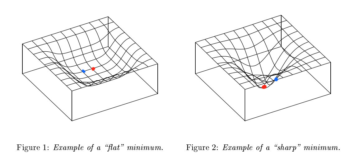Figure [1]: Example of Flat minimum & Sharp Minimum

If you look at Figure 1 in Figure [1], the loss landscape is not deep but flat, and if you look at Figure 2, the loss landscape is deep but narrow. If we calculate the loss at the minima point (red dot) of Figure 1, it will probably be higher than the loss at the minima point of Figure 2. However, even if it deviates slightly from the optimal point during training (blue dot), that is, even if it deviates slightly from the minima, the difference in loss value will not be large because the landscape is gentle.

However, in Figure 2, since the landscape is steep, even a slight deviation from the minima will result in a large difference in loss value. In other words, Figure 1 has a small loss difference between the red dot and blue dot positions, while Figure 2 can be seen as having a large loss difference between the red dot and blue dot positions. Since there is no guarantee that Deep Learning always finds the optimal point during training, it can be seen as more advantageous from a generalization perspective when the loss landscape is made flat.

(However… there is another perspective on whether flatness really has a big impact on generalization; Li, Hao, et al. “Visualizing the loss landscape of neural nets.” Advances in neural information processing systems 31 (2018). Paper )

1.2 SAM Algorithm

Then, how can we make the loss landscape flat? The SAM algorithm finds flat minima through the following 4 steps. (I will omit the proof through formulas.)

1. Calculate Loss: \(\mathcal{L}_\mathcal{B}\)
2. Move in the ”+” gradient direction of the calculated Loss: \(\hat{\epsilon}(w)\rightarrow\) \(w_{adv}=w_t+\hat{\epsilon}(w)\)
   (= Move to the highest Loss)
3. Calculate gradient at the moved position: \(g =\nabla\mathcal{L}_\mathcal{B}(w)|_{w+\hat{\epsilon}(w)}\)
4. Proceed with weight update from the original position: \(w_t=w_t-\eta g\)

*In the case of 2 and 3, the proof is shown in great detail in the paper. During operations including \(\epsilon\), it approximates via Taylor Expansion. Since this is not a SAM paper review… if you are interested, it would be good to look at the paper directly. I will review it if I have a chance next time. (https://arxiv.org/abs/2010.01412)

You can think of the core of SAM as an algorithm based on minmax optimization. Usually, when updating gradients during training, we proceed in the form of \(w = w - \nabla_w{L(w)}\). We update in the opposite direction of the gradient calculated for the Loss. However, in the SAM algorithm, we first move in the positive direction of the gradient. The meaning of this is that even if we give up finding the lowest loss, we will perform the gradient update considering the direction that lowers the highest losses. (Refer to Figure [2])

To explain it a bit more easily and intuitively, it means proceeding with the update while pressing down on the highest losses. It means making the loss landscape generally flat by lowering the high losses rather than finding the low loss.

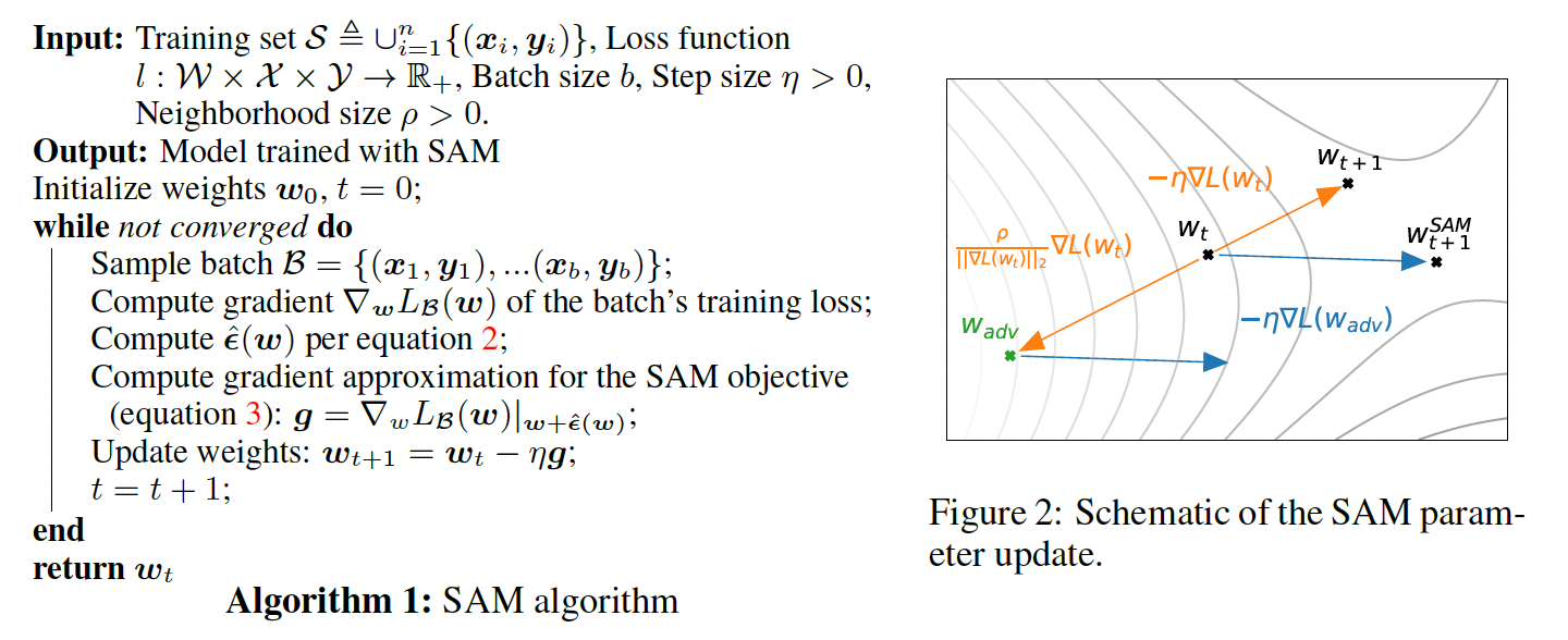Figure [2]: SAM Algorithm

Since SAM is an optimization algorithm rather than a single model algorithm, it can be applied to various models. (Can be used like an optimizer)

2. What is MAML?

MAML (Model-Agnostic Meta-Learning) is a paper written by Professor Chelsea Finn (a PhD student at the time) in 2017, and it is one of the papers that signaled the beginning of Meta-Learning. Since it is such a famous paper, many people probably know it, but I will briefly explain what Meta-Learning is and what kind of algorithm MAML is.

2.1 Meta-Learning

Before that, what is Meta-Learning here? Meta-Learning is one of the fields of few-shot learning. It is a learning method that learns centered on various tasks rather than learning centered on Labels (supervised learning), so that it can classify/predict well even if a completely new task comes in. In other words, it is learning how to adapt to new tasks quickly. (task: Sample extracting K items of N types of data from datasets → N-way K-shot)

Before understanding Meta-Learning, actually, an understanding of few-shot learning must precede. Since the explanation of Few-Shot Learning is well presented in this blog, I will replace it with a link. Here, I think you just need to touch upon the concepts of Support/Query set.

Meta-Learning methods are usually divided into the following 3 types.

• model-based Learning centered on the task’s model
• metric-based (non-parametric) Learning centered on distance in task parameters
• gradient-based (parametric) Learning centered on the gradient of task parameters

As a side note, each method varies depending on the application used.

• In computer vision applications like few-shot classification among Meta-Learning, metric-based learning is often utilized.
• In RL applications like Robotics, model-based learning is often utilized.
• Since Gradient-based learning learns the parameters of the model, it is widely utilized in various fields.

Meta-Learning also has meta-training and meta-validation/test processes.

2.2 MAML

MAML belongs to gradient-based meta-learning among the learning methods classified above. MAML is referenced in most papers related to meta-learning to date because it is extremely simple and convenient to use. As the name MAML suggests, it can be utilized with any model (Model-Agnostic) and can adapt quickly (fast adaptation) to various tasks. The core processes that make up MAML are the following two.

• Calculate loss for tasks through fine-tuning from Initialized $\theta$ (Inner-Loop)
• Gradient update $\theta$ with the calculated loss (Outer-Loop)

Usually, this process is called bi-level optimization.

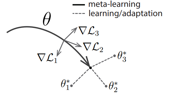
Ultimately, MAML’s final goal is to send the initialized $\theta$ to a position that can cover any task well. To do so, it goes through the two processes mentioned above, which I will explain in detail through the following Figure [3] and notation.

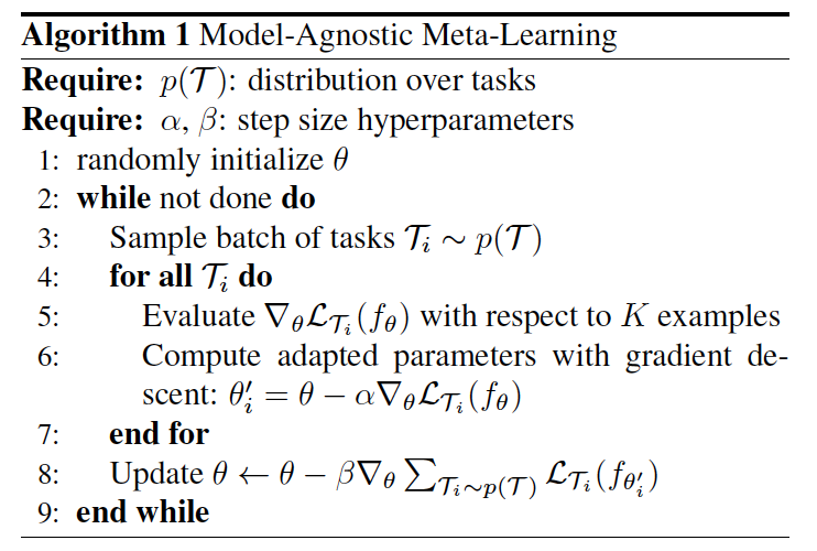Figure [3]: Diagram and Algorithm of MAML

Notation :

• $\mathcal{T_i} = (\mathcal{S_i}, \mathcal{Q_i})$ : (Support, Query) datasets
• $\theta$ : Initialized parameter
• $\theta^\prime$ or $\phi$ : fine-tuned parameter
• $\nabla \mathcal{L_i}$ : gradient of loss from fine-tuned parameter
• (Notation may differ from other blogs and papers.) As mentioned above, to understand MAML, you need to understand two processes: Inner & Outer Loop.

- Inner-Loop & Outer-Loop

First is the Inner-Loop. The Inner-Loop is the process of finding the optimal point for that task through fine-tuning. Expressing this process as a formula, it is $\theta^{\prime} = \theta - \alpha \nabla_{\theta} \mathcal{L}(\theta) $. (Same as step 6 on the right of Figure [3]) This process is identical to Stochastic Gradient Descent. In other words, it is a process of quickly finding the optimal point for that task through SGD. In the MAML paper, this process is performed for 5 steps. Mathematically, from step 2 onwards, in the SGD equation above, it (obviously) changes from $\theta$ → $\theta^{\prime}$. The detailed process of the Inner-Loop is as follows.

1. Sample $\mathcal{T_i}$: ($\mathcal{S_i}$, $\mathcal{Q_i}$) from distribution $\mathcal{p(T)}$
2. Iterate $\theta^{\prime} ← \theta - \alpha \nabla_{\theta} \mathcal{L}(\theta)$ with the $\mathcal{S_i}$ N times (= fine-tuning)
3. Calculate the $\mathcal{L}(\theta^{\prime})$ using the $\mathcal{Q_i}$

To explain the detailed process above easily: fine-tune with the support set, and at the fine-tuned position, check performance with the query set, that is, calculate the loss.

Next is the Outer-Loop. The Outer-Loop is the process of updating $\theta$ with the average of losses calculated in the Inner-Loop. The key here is that the update is done not at the fine-tuned point but at the point where fine-tuning started: $\theta$. Expressing this process as a formula, it is $\theta = \theta - \beta \nabla_{\theta} \sum \mathcal{L}(\theta^{\prime}) $. (Same as step 8 on the right of Figure [3]) The meaning of this formula can be thought of as follows.

1. Use $\mathcal{S_i}$ to provide some information about the corresponding task and train the model. (= Fine-tuning)
2. After Fine-tuning, use $\mathcal{Q_i}$ to evaluate the performance on the corresponding Task and calculate the Loss. (= Calculate Loss)
3. Secure the direction for $\theta$ to learn through the Gradient of the Loss calculated in 2.
4. Update based on the average of gradients of the loss for $n$ tasks. ($i = 1,2,…,n$)

You can think of the gradient of the loss calculated with $\mathcal{Q_i}$ (gradient vector) as informing the direction to update in the future. Since training an unseen-task (here $\mathcal{Q_i}$) from the beginning is difficult and inefficient, we adapt to some extent with $\mathcal{S_i}$, and then train with the gradient that comes out through the unseen task. Unlike supervised learning which learns individual tasks or data one by one, it can be seen as learning the method to go to the optimal point. When this happens, since it is not learning on specific data, overfitting does not occur easily, and it also has strengths in generalization as it can quickly adapt to unseen-tasks.

However, in this case, there is a disadvantage that the computational cost is slightly high because differentiation is performed twice (Inner-Loop differentiation, Outer-Loop differentiation $\rightarrow$ Hessian).

From now on:
Inner-Loop = Fine-tuning
Outer-Loop = Meta-update

3. Sharp-MAML?

You can consider the Sharp-MAML paper as a combination of SAM and MAML described above.

3.1 Problem Formulation & Algorithm

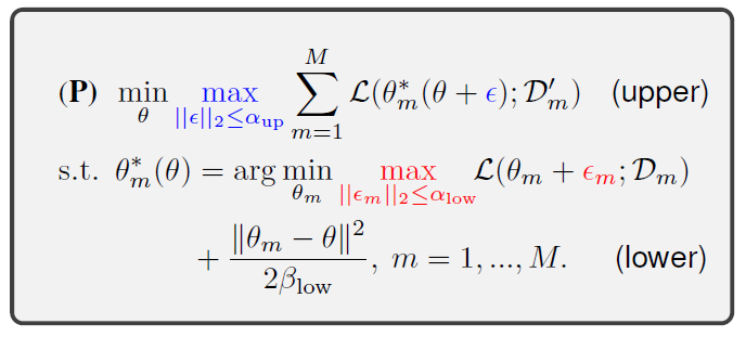
1. Apply only during Fine-Tuning: $\alpha_{up} = 0$ & $\alpha_{low} > 0$
2. Apply only during Meta-update: $\alpha_{up} > 0$ & $\alpha_{low} = 0$
3. Apply Both: $\alpha_{up} > 0$ & $\alpha_{low} > 0$

Figure [4]: Problem formulation of Sharp-MAML

Before diving in!!

• In this paper, the Taylor approximation defined in SAM is defined as biased mini-batch gradient descent (BGD). (at point: $\theta + \epsilon + \epsilon_m$)
• BGD$(\theta,\epsilon, \epsilon_m) = \theta + \epsilon - \beta_{low} \nabla \mathcal{L}(\theta + \epsilon + \epsilon_m) $

If you look at the right side of Figure [4], you can see how SAM was applied to MAML; it was applied in a total of 3 ways: fine-tuning, meta-update, and Both. First, let’s look at the lower part. The author of the paper gives perturbation to the surroundings at every one-step update during fine-tuning to find the high loss and proceeds in the direction of lowering that loss based on it. The formula in the paper is as follows.

• For each task m…
• perturbation: $\epsilon_{m}(\theta) = \alpha_{low} \nabla \mathcal{L}(\theta) / ||{\nabla \mathcal{L}(\theta)}||_{2}$
• maximum point (=maximum loss): $\theta + \underset{||\epsilon_m||_{2} \leq \alpha_{low}}{\max} \epsilon_{m}(\theta)$
• gradient descent: $\tilde{\theta^1} = BGD(\theta, 0, \epsilon_m) = \theta -\beta_{low}\nabla \mathcal{L}(\theta + \epsilon_{m}(\theta))$
• regularizer term: $\frac{|| \theta_m - \theta ||}{\beta_{low}}$

Next is the upper part. Here too, we give perturbation to find the highest loss within that range and proceed in the direction of lowering that loss. The difference is that when giving perturbation, we utilize the gradient calculated during fine-tuning. The formula in the paper is as follows.

• (meta) perturbation: \(\epsilon(\theta) = \alpha_{up} \nabla \mathcal{h} / \|\mathcal{h}\|_2\)(→\(\nabla \mathcal{h} = \nabla_{\theta} \sum_{m=1}^{M}\mathcal{L}(\tilde{\theta^1})\))
• maximum point: $\theta + \underset{||\epsilon_m||_{2} \leq \alpha_{low}}{\max} \epsilon_{m}(\theta) + \epsilon(\theta)$
• gradient descent: $\tilde{\theta^2} = BGD(\theta, \epsilon, \epsilon_m) = \theta + \epsilon - \beta_{low} \nabla \mathcal{L}(\theta + \epsilon + \epsilon_m)$
• meta-update: $\theta \leftarrow \theta - \beta_{up} \sum_{m=1}^M \nabla_{\theta}\mathcal{L}(\tilde{\theta^2}) $

Showing the above process in Pseudo-Code is like Figure [5].

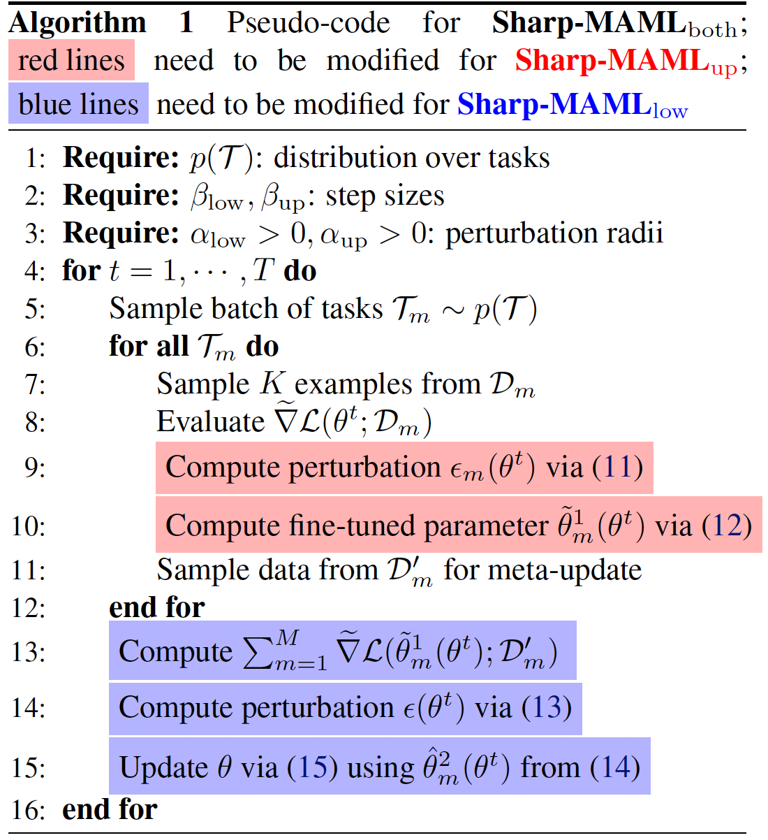Figure [5]: Pseudo-Code for Sharp-MAML

3.2 Results

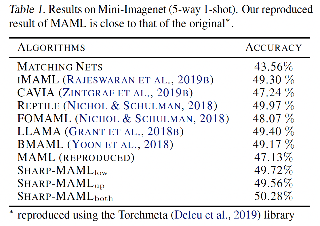
The results are as follows.

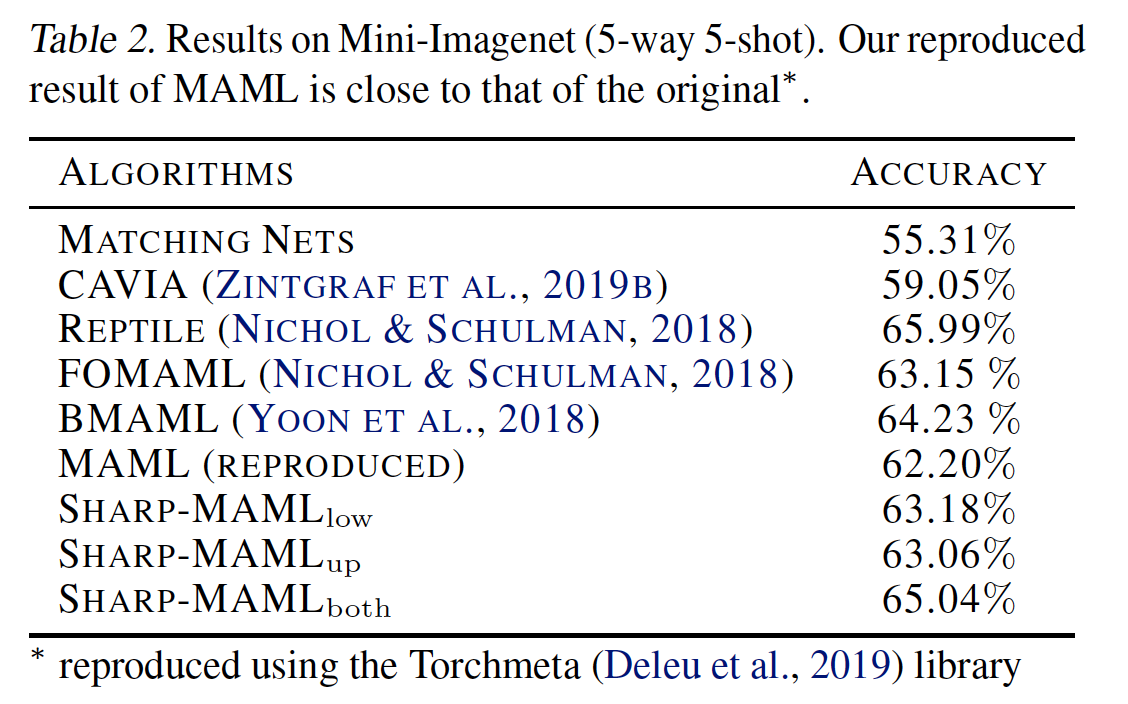Figure [6]: Results of Sharp-MAML

It was somewhat disappointing. There is a gain of about 2~3%, but compared to meta-learning papers coming out these days, it is not a huge gain. Actually, when I first read this paper (around May 2022 last year…), the result in the officially published paper was around 60% based on 5way-1shot, but when I looked it up again recently, it had changed to 50%. In terms of Novelty, there is definitely a contribution, but since the results are not outstanding, I think it would have been a more excellent paper if there were more gains. Also, if they wanted to emphasize generalization more, I wonder how it would have been if results for cross-domain adaptation were also included.

Finally, let’s briefly examine what significance Sharp-MAML has along with its loss landscape. (Subjective thoughts are also included.)

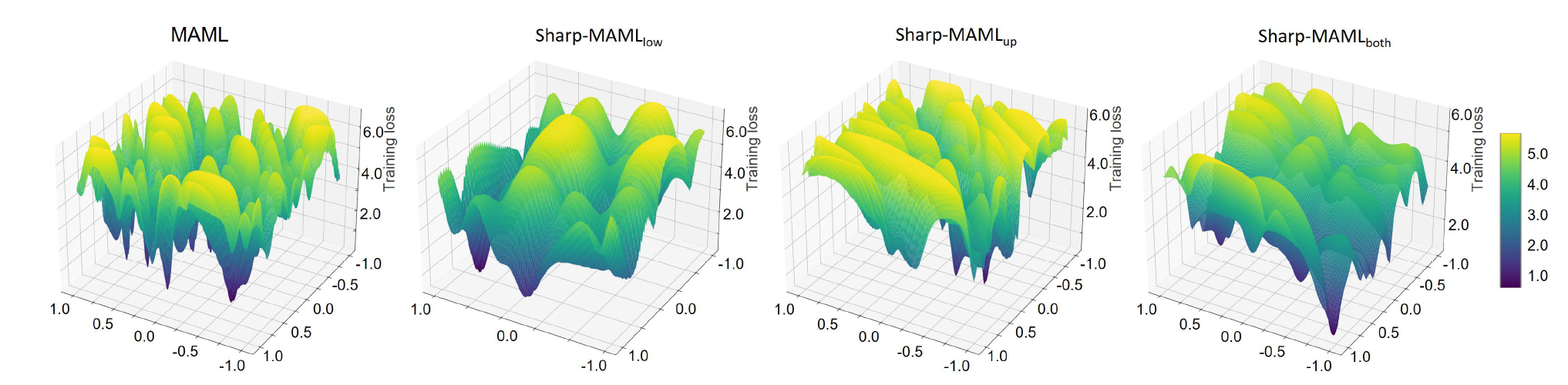
Figure [7]: Loss Landscape of Sharp-MAML

Looking at Figure [7], you can see it has become fairly flatter than the existing MAML. The MAML paper said it had strengths in generalization, so I was curious, “Is MAML also flat?”. However, it was not very flat on the loss landscape. Then, we can think, “Does generalization increase if MAML’s loss landscape becomes flatter?”, and Sharp-MAML showed those results. If we think carefully, when the loss landscape is flat, the possibility of various tasks falling into local minima during fine-tuning or meta-update decreases, so we can think that the possibility of generalization increasing rises.

4. Conclusion

Just as I was getting interested in Flatness while studying Meta-Learning, the Sharp-MAML paper came out. It was impressive to see them trying to solve MAML with flatness while looking at it from a generalization perspective. However, since it is gradient-based, no matter how good the novelty is, it seems insufficient to overcome the limitations of the black-box (?) yet, and much research seems necessary. For those who want to check the novelty of this paper more, it would be good to read the theoretical analysis part or the appendix in the paper.

5. Reference

• Abbas, Momin, et al. “Sharp-MAML: Sharpness-Aware Model-Agnostic Meta Learning.” International Conference on Machine Learning. PMLR, 2022. (Paper)
• Finn, Chelsea, Pieter Abbeel, and Sergey Levine. “Model-agnostic meta-learning for fast adaptation of deep networks.” International conference on machine learning. PMLR, 2017. (Paper)
• Foret, Pierre, et al. “Sharpness-aware minimization for efficiently improving generalization.” arXiv preprint arXiv:2010.01412 (2020). (Paper)
• Li, Hao, et al. “Visualizing the loss landscape of neural nets.” Advances in neural information processing systems 31 (2018). (Paper)