[Theoretical Background] Convex Optimization 1

$\star$ First, before explaining, I will skip the basics of convex and non-convex functions, as well as the general formulas used in deep learning. They are explained so well in other blogs, so is there a need to repeat them? Instead, I will focus more on “Why?” and “How?” In particular, I will focus on the formula derivations.

Why Convex Optimization?

Most problems we actually need to solve are non-convex. However, solving non-convex functions requires more careful approximation and proof, which can make the process expensive and inefficient. If we instead assume that the function is convex within a reasonable range, we can solve it more efficiently. In other words, if we assume that an arbitrary function $f$ is convex, the local minimum of $f$ is also the global minimum. The problem becomes relatively easy because we only need to find a local minimum. Let’s look at this through some simple examples.

The Taxonomy below represents the classification criteria used in optimization. $\star$ Taxonomy:

• Zeroth Order: Only the function value
• $1^{st}$ Order: Derivatives (GD/SGD/mini-batch GD, etc.)
• $2^{nd}$ Order: Hessians (Newton methods, etc.)

Example: Gradient Descent

One of the most basic methods for finding an optimal solution in the Deep Learning field is Gradient Descent (hereinafter, GD). Nowadays, most people use other optimization techniques (e.g., SGD, Adam, etc.) instead of plain GD. However, if you understand how GD converges from an optimization perspective, I think you will be able to understand the other techniques more easily as well.

Then, let’s look at how optimization is performed with GD and how the convergence behavior changes according to the assumptions. (All assumptions here are based on convexity.)

Problem Formulation 1
(Assumption: $L$-Lipschitz)

Before we dive in, let us briefly establish the optimization setting:

where $f$ is a differentiable convex function.

Since GD is an iterative algorithm, it can be written as follows:

​ where $\gamma > 0 $ is the step size, also known as the learning rate.

To find the optimal solution, we repeatedly apply the update above. Assuming that training does not diverge, the quality of an optimization algorithm depends on how quickly it finds the optimal solution. So, how do we measure this? We can use an upper bound based on the final step $T$. In other words, after training has proceeded for $T$ steps:

Theorem 1: Let $f$ be convex and $L$-Lipschitz continuous. Then gradient descent with $\gamma = \frac{\mid\mid x_1 - x^\star\mid\mid}{L\sqrt{T}}$ satisfies:

Proof:

First, to solve the problem, we can use a method based on projection onto convex sets. In other words, when projecting onto a convex set, the inner product involving $x$, $z$, and the projection point $\pi_c (z)$ always results in a non-positive value (an obtuse angle), and the Pythagorean theorem gives the inequality $\mid\mid \pi_c (z) - x\mid\mid \leq \mid\mid z - x \mid\mid$. Later in the proof, I will also use the following form of the Pythagorean theorem: $\mathbf{\left<a,b\right> = \frac{1}{2}(\mid\mid a\mid\mid^2 + \mid\mid b\mid\mid ^2 -\mid\mid a-b\mid\mid ^2)}$)

Using the properties above, let’s develop the proof:

Here, the $L$-Lipschitz continuity property tells us that if $f$ is differentiable, then $\mid \nabla f (x) \mid \leq L$. Using $\frac{\gamma}{2} \mid\mid \nabla f(x_k)\mid\mid ^2 \leq \frac{\gamma L^2}{2}$, we can set the following bound.

Now, let’s substitute the values of $k$ sequentially and expand the formula.

If we take the average of both sides of the inequality:

Here, since $\mid\mid x_{T+1} - x^\star\mid\mid ^2$ has a minus sign in front of it, this term is always non-positive. Therefore, we can drop it and obtain an additional upper bound.

And then, *using Jensen’s Inequality, we can write $f(\frac{1}{T} \sum_{k=1}^Tx_k) \leq \frac{1}{T} \sum_{k=1}^Tf(x_k)$. (This follows from our assumption that $f$ is convex.)

*Jensen’s Inequality: If $f$ is convex, then it satisfies $f(\mathbb{E}[x])\leq \mathbb{E}[f(x)]$.

Substituting this into the bound gives:

Finally, if we substitute the step size $\gamma = \frac{\mid\mid x_1 - x^\star\mid\mid}{L\sqrt{T}}$,

After expanding the expression, we obtain exactly the result in Theorem . This means that the convergence rate depends on $T$. Assuming that $f$ is convex and $L$-Lipschitz, the convergence rate is $\mathcal{O}\left(\frac{1}{\sqrt{T}}\right)$.

Side Note: Fixed Step Size vs. Adaptive Step Size

If you look at other textbooks, papers, and blogs, you will often see a fixed step size $\gamma = \frac{1}{L}$ used when proving the convergence of Gradient Descent. This approach is mathematically neat, and the convergence rate is also faster at $\mathcal{O}(\frac{1}{T})$. However, because the step size is fixed, expanding the formula creates a term in the right-hand-side bound that is independent of $\frac{1}{T}$. Therefore, we cannot guarantee that the bound actually approaches the minimum. You can understand the method developed here as giving up some convergence speed in exchange for a more adaptive step size, which depends on the difference between the initial input $x_1$, the optimum $x^\star$, and the number of iterations $T$.

(Since proofs for the fixed-step-size case are widely available, I will omit them.)

Afterwards…

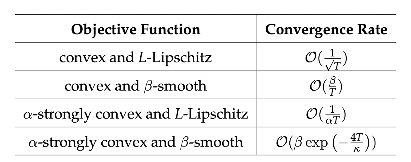
The derivation above was developed under the assumption that $f$ is convex and $L$-Lipschitz continuous. If the assumptions become stronger ($\beta$-smooth, $\alpha$-strongly convex, etc.), the convergence rate changes. In future posts, I will derive the convergence rate under different assumptions.

I will finish by introducing a convergence-rate table for GD under different assumptions.

$*$Thank you very much for reading. If you find any incorrect parts or have any advice, I would appreciate it if you shared your thoughts anytime.​