[Conceptual Background] Meta Learning (2) - Approaches

2. Meta Learning Approaches

Actually, the reason I explained Few-Shot Learning in the previous post was to help explain Meta-Learning. You can understand Meta-Learning as applying various approaches based on the concept of Few-Shot Learning. Without further ado, let’s see what approaches exist in Meta-Learning.

Meta-Learning can basically be classified into the following three broad categories:

• Optimization-based Approach
• Metric-based Approach
• Model-based Approach

I will explain the key approaches and important papers for each category. However, I will skip the model-based approach here. Since model-based approaches are often used in RL, I will post about them separately next time if I have the chance.

It would be good to check how $S$ and $Q$ are utilized for training while reading.

2.1 Optimization-based Meta Learning

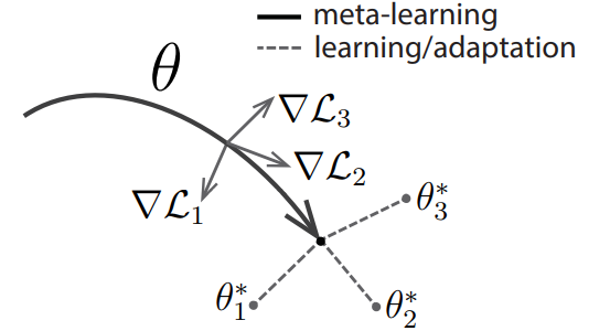
Optimization-based Meta-Learning is a method centered on learning through gradients. The first paper to discuss here is Model-Agnostic Meta-Learning (MAML), which was published in 2017. It is essentially the paper that popularized the concept of “Meta-Learning.” So, let’s examine what kind of paper MAML is.

2.1.1 MAML

The final goal of MAML is to train the model parameter $\theta$ to a position where fast adaptation or fine-tuning (hereinafter FT) is possible. The key idea is: “It would be efficient if we could reach specific tasks through only a few parameter updates!” Let me explain with an example. If a person has a job that requires traveling all over the country (Korea), it would be more efficient to live in Daejeon (the central region) than to live in Busan, Gangneung, or Incheon. Similarly, moving $\theta$ to a position from which it can quickly reach many tasks is better for achieving good performance across various tasks than learning every task individually.

While the paragraph above explained the idea in words, let’s look at it mathematically this time. Before diving in, MAML is divided into an inner-loop and an outer-loop during each training epoch. The inner-loop is the FT mentioned above, and the outer-loop is the model update$^*$. The MAML algorithm is shown in Figure 1.

$^*$ Usually, this process is also called bi-level optimization.

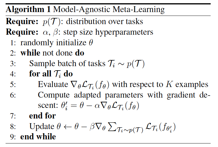Now, let’s explain the pseudo-code above in detail:

1. Initialize model parameter $\theta$ (line 1)
2. Sample task $\mathcal{T}$ =($S$,$\mathcal{Q}$ ) ; $\mathcal{T} \sim p(\mathcal{T})$ along with the number of batches (line 3)
3. Inner-Loop updates with $n$ steps (line 4-7):
   1. Repeat SGD update: $\phi = \theta - \alpha\nabla_\theta \mathcal{L}(S;\theta)$
   2. From $n \geq 2$, it changes from $\theta$ → $\phi$; i.e., update in the form of $\phi = \phi - \alpha \nabla_\phi \mathcal{L}(\mathcal{S}; \phi)$
4. Outer-Loop (line 8):
   1. With fine-tuned model $\phi$, evaluate with $\mathcal{Q}$ and update
   2. $\Rightarrow$ $\theta \leftarrow \theta - \frac{1}{N}\sum_{i=1}^N \nabla_\theta \mathcal{L}_i(\mathcal{Q};\phi) $
5. Repeat 2-4 (line 2-9)

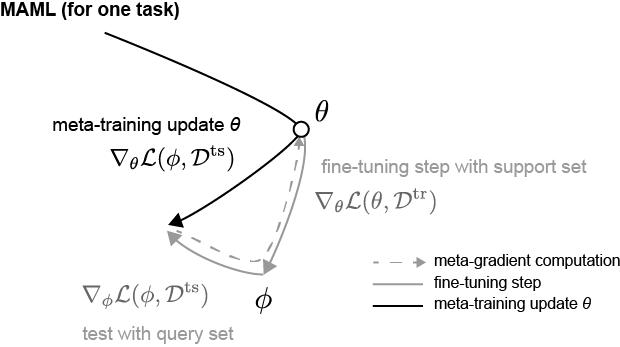
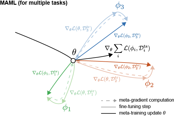
The important point here is the derivative (meta-gradient) during the outer loop. When performing the outer-loop update, we differentiate with respect to $\theta$, not $\phi$, even though the loss is calculated using the fine-tuned parameter $\phi$ and $Q$. The related formula can be expanded using the chain rule as follows.

The purpose of this formula is ultimately to update $\theta$ toward a lower loss, specifically in a direction that lowers the loss $\mathcal{L}(\mathcal{Q};\phi)$ at the fine-tuned $\phi$. This might feel ambiguous, but looking at Figure 2 may help you understand the direction of the update. (Reference: Boyang Zhao’s Blog. The notation is slightly different, but you can simply interpret it as the loss.)

2.1.2 FOMAML, Reptile

In MAML, Hessian matrix multiplication ($=\nabla_\theta^2 \mathcal{L}(\mathcal{S};\phi)$) is included, which creates a computational cost. Therefore, methods were proposed to reduce the cost while maintaining performance to some extent.

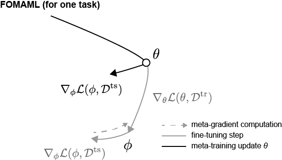
One of them is FOMAML (First-Order MAML). The MAML paper experimentally showed that FOMAML maintains performance to some extent even when training proceeds while ignoring the Hessian matrix. In other words, it assumes $\nabla_\theta^2 \mathcal{L}(\mathcal{S};\phi) = 0$. This is illustrated in Figure 3: it applies to $\theta$ the “direction of the gradient” that lowers the loss $\mathcal{L}(\mathcal{Q};\phi)$ at the fine-tuned $\phi$. The paper explains that this mechanism is possible because the Hessian value converges to 0 when passing through ReLU. From a Loss Landscape perspective, the “direction that lowers the loss” is similar. In other words, it implicitly assumes that the final updated $\theta$ position in MAML and the $\theta$ position in FOMAML lie in similar loss landscapes.

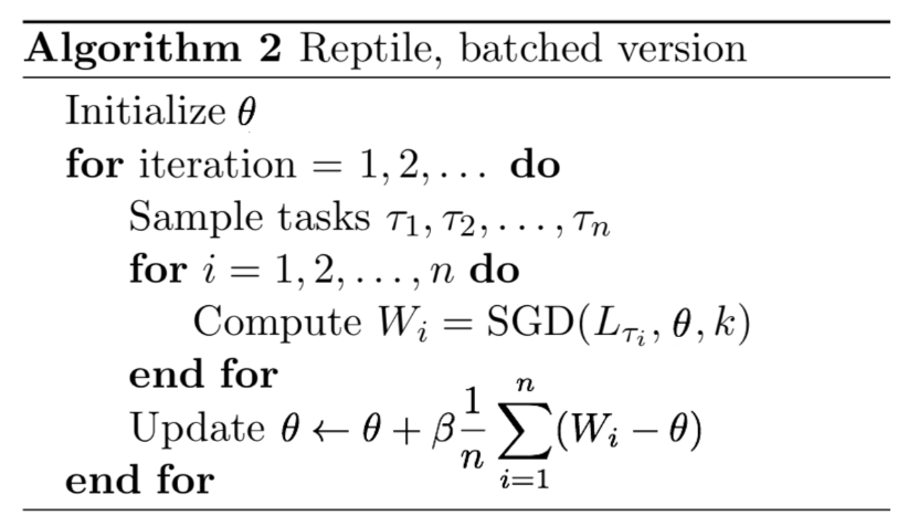
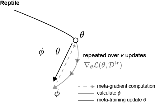
Next is the Reptile paper. The Reptile paper was published by OpenAI in 2018, and you can think of it as a variant of FOMAML. The characteristic of Reptile is that $S$ and $Q$ do not exist separately. It uses a few-shot setting, but samples multiple tasks and trains on the selected tasks. It then updates the model using the difference between the initial model parameter $\theta$ and the fine-tuned model parameter $\phi$ as the gradient. Figure 4 below shows the Reptile algorithm and its update direction.

The notation may be different from the original MAML paper, which can be confusing, so the process is explained in detail below:

1. Initialize model parameter $\theta$
2. Pick $N$ Tasks $\mathcal{T}_i$. (where $\mathcal{T}_i \sim p(\mathcal{T})$, batch = $N$)
3. Inner Loop: FT for each task $\mathcal{T}_i$ (fine-tuned parameters: $\phi_i$)
4. Outer Loop: Update $\theta$ by the difference between $\theta$ and $\phi$: $\theta \leftarrow \theta + \frac{\beta}{N}\sum_{i=1}^N (\phi_i - \theta)$
5. repeat 2-4

When trained this way, the expected meta-gradient in the Reptile algorithm ultimately converges to something similar to the meta-gradient of MAML. Most of the Reptile paper is devoted to mathematically proving why it converges similarly to MAML and FOMAML. However, here we will only look at the broad idea. I will also make a post related to the proofs if I have the chance someday.

2.1.3 Wrap-up

Optimization-based Meta-Learning is an approach that uses gradients for training in a few-shot setting. Unlike other approaches, it has the advantage that, when the gradient-based update is designed appropriately, it can be applied in a model-agnostic way across various fields. In other words, it can be used in fields such as regression, classification, and reinforcement learning.

2.2 Metric-based Meta Learning

Metric-based Meta-Learning is an approach that trains by calculating similarity based on distance. Simply put, each class has semantic information, and training proceeds by measuring the similarity between those representations. In a way, it is similar to the nearest-neighbor concept used in $k$-NN. Representative examples include Matching Network, Prototypical Network, and Relation Network, and we will examine the main concepts discussed in each paper. (It would be good to keep the concept of Few-Shot Learning in mind.)

2.2.1 Matching Network

The first paper to look at is Matching Network, a pioneering paper in the metric-based approach. Thinking about the context at that time, the seq2seq paper, which later became one of the foundations of the Transformer, had emerged. It focused on learning from the overall context rather than looking only at extracted features through the Attention mechanism. Therefore, the Matching Network paper aimed to compare the context between features produced by an encoder.

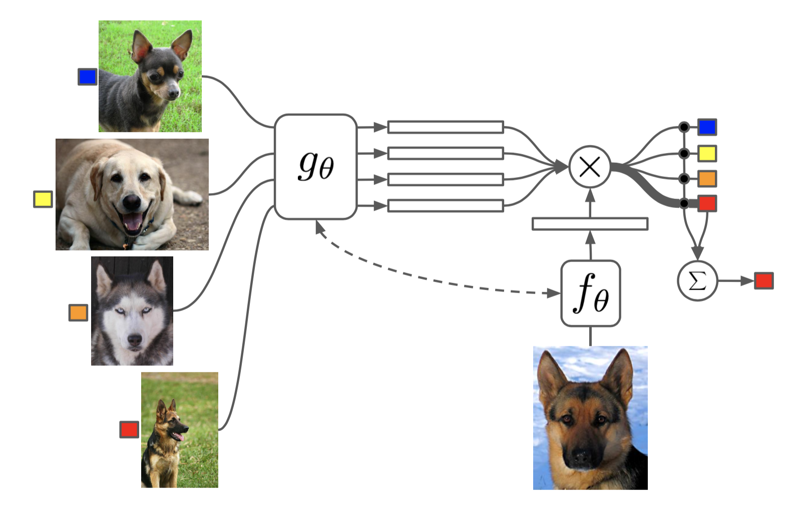
First, before explaining the training process, this paper explains the final output.

The formula above shows that the attention mechanism is used to assign different weights to the support samples. Here, $a(\cdot, \cdot)$ is the attention kernel, which applies a softmax to the cosine similarity:

In simple terms, we calculate the similarity between each support sample $\textbf{x}_i $ and the input $\textbf{x}$ using the attention kernel. We then use the similarity as a weight, so the prediction is biased toward the class with higher similarity. Here, you can understand the input $\textbf{x}$ as a query sample.

Now, let’s look at the training process using the notation below.

1. Extract feature representation vector of support set through $g_\theta$
2. Extract feature representation vector of query set through $f_\theta$ (Usually $f_\theta = g_\theta$)
3. Calculate attention value between feature representation vectors from 1 and 2 $\rightarrow a(\cdot, \cdot)$
4. Predict label of query set through $C_\mathcal{S}$

Unlike more recent papers, early Meta-Learning papers often used LSTM structures to handle the few-shot setting from a contextual perspective. Therefore, this paper also proposed an additional method using an LSTM structure ($\rightarrow$ Full Context Embeddings; FCE). Let’s look at the FCE training process and how the LSTM architecture is used.

• Embedding $g$
  • $g \rightarrow $ bidirectional LSTM, $g’ \rightarrow$ CNN (feature extractor)
  • $g(x_i, \mathcal{S})= \overrightarrow{h}_i + \overleftarrow{h}_i + g^\prime (x_i) $
  • $\overrightarrow{h}_i,\overrightarrow{c}_i = \text{LSTM}(g^{\prime} (x_i), {\overrightarrow{h}}_{i-1}, {\overrightarrow{c}}_{i-1})$ , $\overleftarrow{h}_i,\overleftarrow{c}_i = \text{LSTM}(g^{\prime} (x_i), {\overleftarrow{h}}_{i+1}, {\overleftarrow{c}}_{i+1})$
• $f \rightarrow$ LSTM , $f’ \rightarrow$ CNN (feature extractor)
  • $f(\hat{x}, \mathcal{S}) = \text{attLSTM}(f^\prime(\hat{x}), g(\mathcal{S}), K) $

$\Rightarrow$ According to $k$ step…

1. $\hat{h}_k, c_k = \text{LSTM}(f^\prime (\hat{x}), [h_{k-1}, r_{k-1}], c_{k-1}) $​
2. $h_k = \hat{h}_k + f^\prime(\hat{x})$
3. $r_{k-1} = \sum_{i=1}^{|\mathcal{S}|}a(h_{k-1}, g(x_i))g(x_i)$
4. $a(h_{k-1}, g(x_i)) = \text{softmax}(h^\text{T}_{k-1}g(x_i))$

Ultimately, the reason for using an LSTM here is to better capture the context of each feature vector. On easier tasks like Omniglot, there is not much performance gain, but on slightly more difficult tasks like $mini$-ImageNet, there is a performance gain.

2.2.2 Prototypical Networks

The next paper is Prototypical Networks (hereinafter ProtoNet). In fact, you can think of much of the later metric-based Meta-Learning research as being based on ProtoNet rather than Matching Network.

I’ll get straight to the point. ProtoNet trains by calculating the Euclidean distance between the prototype vector of each label and the feature vectors. Looking at Figure 6 below, $c_n$s represent the prototype of each label. For a new task, the model calculates the distance to each prototype and assigns the sample to the label of the closest prototype. The prototype is obtained by averaging the feature vectors derived from the Support set. Now, let’s look at the training process in more detail.

• Notation (I will explain as similarly to the paper as possible):
  • Support Set $\mathcal{S}_{n}= \{ (x_{n,j}^s, y_{n,j}^s) \}_{j=1}^{K}$, Query Set $\mathcal{Q}_{n}= \{ (x_{n,j}^q, y_{n,j}^q) \}_{j=1}^{Q}$​
  • $K$: number of support set (a.k.a $K$-shot)
  • $Q$: number of query set
  • $c_n$: prototype of label $n$ $\rightarrow$ $\{c_1,\dots,c_N \}$, ($N$: $N$-way)
  • $f_\theta$ : Model parameterized by $\theta$​ (hereinafter feature extractor or backbone network)
  • loss $\mathcal{L}(\mathcal{D},c,\theta) = \frac{1}{|\mathcal{D}|}\sum_{(x,y)\in \mathcal{D}} l(-d(f_\theta(x), c),y)$,
    $\rightarrow$ loss function $l(\cdot, \cdot)$: Cross Entropy (CE), $-d(\cdot, \cdot)$: Euclidean Distance

1. $c_n = \frac{1}{| \mathcal{S}_n |} \sum_{j=1}^{| \mathcal{S}_n |} f_\theta (x^s_{n, j}) \Rightarrow $ Calculate prototype vector ${c_n}$ with support set
2. $\sum_{n=1}^{N}\mathcal{L}(Q_{n}, c_n, \theta) \Rightarrow$ Calculate Euclidean distance between query set and prototype $c_n$​
3. $\theta \leftarrow \theta - \nabla_{\theta}\sum_{n=1}^{N}\mathcal{L}(Q_{n}, c_n, \theta)$ $\Rightarrow$ model parameter update

Since there is quite a lot of notation and it is complex, the process may be difficult to understand at first. If it feels complicated, it may be helpful to think of it simply as follows:

• Create a prototype for each label using the Support Set.
• Compare the Query Set with the prototypes $\Rightarrow$ Logits (final output).
• Calculate the CE between the Query Set labels and the logits.
• Update the parameters using the CE loss.

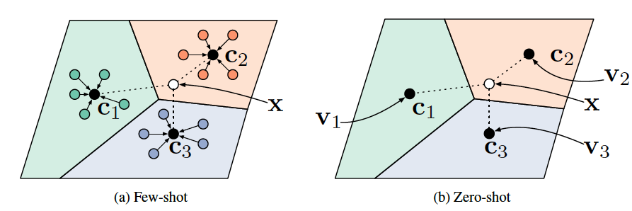
This paper does not use a linear layer. Since the feature vectors are directly used to calculate distances, a separate linear layer is not used even though this is a classification task. However, the paper explains that Euclidean distance can be reinterpreted as a linear model. I will explain this using the following two formulas.

This is the reason why ProtoNet chose Euclidean distance over other distance metrics. The basic idea in Deep Learning is that, if the backbone network learns a good feature representation, the remaining step only requires a suitable linear transformation, especially for classification tasks. Usually, this is implemented by attaching a learnable linear layer behind the backbone network. However, ProtoNet interprets training through Euclidean distance as an implicit linear transformation. Another reason Euclidean distance may be appropriate is that the parts requiring non-linearity are assumed to have already been learned by the backbone network. In fact, this assumption comes from a familiar structure: backbone model → linear layer. The paper seems to mention this because deep learning research was not as extensive at that time.

(Really lastly…) Another advantage of this reinterpretation is that MAML (hereinafter Proto-MAML) can be applied to ProtoNet. Since $w_k^{\text{T}}f_\theta(x) +b_k$ acts as a linear layer, FT becomes possible. I will briefly explain the Proto-MAML training process.

• Notation:
  • $f_\theta$: backbone network
  • $g_\theta(x_i) = w_{i,k}^{\text{T}}f_\theta(x_i) +b_k$
  • Loss $\mathcal{L}(\mathcal{D};\theta) = \frac{1}{|\mathcal{D}|}\sum_{(x,y)\in\mathcal{D}}l(g_\theta(x), y)$

1. Inner Loop 1. Calculate prototype $c_{i,k}$ through support set $\mathcal{S}_i$
   1. $\phi = \theta - \alpha \nabla_\theta \mathcal{L}(\mathcal{S}_i;\theta)$
   2. Repeat $n$ steps
2. Outer Loop: $\theta \leftarrow \theta - \frac{\beta}{\mathcal{B}}\sum_{i=1}^{\mathcal{B}}\nabla_\theta \mathcal{L}(\mathcal{Q}_i;\phi)$

There is also a paper that proposed (fo-)Proto-MAML. Although it is not the main focus of the paper, the authors showed that Proto-MAML provides a performance gain.

*Conclusion

Up to this post, I think I have covered most of the pioneering papers in Meta-Learning. Research on Meta-Learning grew rapidly for about 4–5 years after the papers mentioned above appeared in 2016 and 2017. Although the pace has slowed slightly, research in this area is still consistently published at top conferences. However, the trend has changed from studying Meta-Learning algorithms themselves to applying them to other research areas. In particular, as foundation-model research becomes increasingly active, the concept of Few-Shot Learning, which allows models to learn from a small amount of data, seems to have become even more important.

For the next topic, I am thinking about posting either paper reviews or conceptual articles on foundation models (LLM, LVM, etc.), which I have only recently started studying. I am not sure which specific direction to take yet, but I will return after studying them a bit more. Thank you for reading.