[Conceptual Background] Rethinking on Weight Decay

Recap of Weight Decay (WD)

Recently, when training models, we mostly use Weight Decay (WD). There are many benefits to using WD, and a representative effect is preventing overfitting. Then, what is WD, and how can it prevent overfitting?

Generally, when encountering Deep Learning for the first time, you probably learn WD as follows:

In other words, when training through the Loss Function as shown above, we train in a direction that reduces the norm value of the model’s weight parameter in addition to the existing derived loss. When this happens, intuitively, it sends most weight parameters close to 0, reducing the model’s complexity, and through this, we can see the effect of preventing overfitting.

However, here we need to examine the role of WD a bit deeper. The reason is that the role of WD is not limited simply to ‘preventing Overfitting’. For example, recently WD is essentially applied even to very large models like LLMs. If you think about it, since LLMs are trained for about 1 epoch on very large datasets, there is essentially no need to consider overfitting. Nevertheless, we often proceed by applying an (even) larger WD ratio $\lambda$.

Therefore, in this post, I will try to explain the role of WD and its significance as I see it.

1) WD is actually a Prior Knowledge Distribution!

There is one ‘representative assumption’ that is commonly used when doing statistical modeling in the deep learning field. When we define a distribution, we often assume that it follows the Gaussian Distribution, because it is the easiest to handle. The reason is simple: the normal distribution can fully describe an entire distribution using only its Mean and Variance, without requiring complex parameters. Therefore, before I go into the full explanation, I will also make the following assumption:

Assumption: Model weight parameters follow a Gaussian distribution.

If this assumption holds, we can make the following statement:

WD is a Maximum A Posteriori (MAP) estimation assuming the weights have a Gaussian prior.

Let’s take a closer look at what this means. Here, rather than looking at deep learning training from an optimization perspective, we will look at it from a probability perspective of finding the optimal solution.

(I wrote this section by synthesizing the contents of PRML Chapter 3.3 and various other materials.)

Expansion of concept from MLE to MAP

Usually, when we train a model, we try to find the model parameter $\theta$ that minimizes the Loss Function (e.g., MSE, CE). In statistical terms, this is called Maximum Likelihood Estimation (MLE). MLE is an estimation method from the data perspective; simply put, it means “Let’s estimate $\theta$ so that we can maximize the probability $p(\mathcal{D} \mid \theta)$ of observing the given dataset $\mathcal{D}$”. Expressing MLE as a formula gives us:

I think most of you are familiar with this formula. It is essentially the Loss Function we usually use. That is, if we convert the above MLE into a minimization problem by attaching a negative sign, it becomes the Loss Function $\mathcal{L}(\theta)$ we usually use.

(Returning to the main point) However, although MLE is the most universal approach, it has one downside: it relies entirely on the observed dataset $\mathcal{D}$. Let me explain with an example. Let’s say we found the optimal $\theta^\ast$ for a specific dataset $\mathcal{D}_1$. Even if this $\theta^\ast$ is optimal for $\mathcal{D}_1$, it might not be the optimal solution for a new $\mathcal{D}_2$ whose data distribution is slightly different. In other words, when the given data is too small or biased, MLE can excessively fit the characteristics (even the noise) of that data. This becomes the fundamental cause of what we commonly call overfitting.

To prevent overfitting, what if we make an assumption (prior) about $\theta$ before seeing $\mathcal{D}$? In other words, if we proceed with training by looking only at $\mathcal{D}$, the model may deviate too much from that data distribution. So, what if we define the $\theta$ we want to find in advance, before seeing $\mathcal{D}$? Here, we view this from a Bayesian perspective. That is, we consider a prior for $\theta$ before seeing $\mathcal{D}$, and this is called Maximum A Posteriori (MAP) estimation. Expressing this as a formula gives:

Here, $p(\theta \mid \mathcal{D})$ can be expanded as follows by Bayes’ theorem:

The equation above becomes a problem of maximizing the product of $p(\mathcal{D}\mid \theta)$ (Likelihood) and $p(\theta)$ (Prior). Since $p(\mathcal{D})$ can be treated as a known constant, we do not need to consider it. Now, how can we treat $p(\theta)$ as a prior and solve the problem?

Prior Knowledge: Gaussian Prior $\mathbf{\theta}$

Now, let’s apply the assumption about the Gaussian prior mentioned earlier. If $p(\theta)$ follows the standard $\mathcal{N}(0, \sigma^2)$ distribution, $\theta$ can be expressed with the following relation:

Let’s substitute this assumption into the MAP equation. To simplify the calculation of the product form, let’s take the log of both sides and attach a negative sign again to convert it into a minimization problem. Then, it becomes as follows:

If we rearrange the equation above, the $\log$ and $\exp$ terms disappear, and we get the following:

Looking at this equation, it is very similar to the WD Eq.\eqref{eq:weight_decay} summarized above. Here, only the coefficients—$\frac{\lambda}{2}$ in Eq.\eqref{eq:weight_decay} and $\frac{1}{2\sigma^2}$ in Eq.\eqref{eq:map_min}—are different, but the form is exactly the same. In other words, if $\lambda = \frac{1}{\sigma^2}$, they can be considered perfectly equivalent.

Meaning of WD Ratio $\lambda$

The WD we conventionally use is not just a simple technique. We can also understand it through the idea that the weight parameter follows a Prior Distribution modeled by $\mathcal{N}(0, \sigma^2I)$ (Eq. $\eqref{eq:prior_gaussian}$).

More importantly, $\lambda$ and variance $\sigma^2$ are inversely proportional. Usually, when $\lambda$ is set too large, training may not converge. On the other hand, when $\lambda$ is set too small, we do not see the full effect of WD. Let’s think about these cases together with variance $\sigma^2$ to understand why this happens:

• $\lambda \uparrow$ $\Rightarrow$ $\sigma^2 \downarrow$ : A small variance in the Prior Distribution means that the variables are heavily concentrated around 0. In this case, if the dataset $\mathcal{D}$ has a broad distribution, it is difficult to find the optimal $\theta$.
• $\lambda \downarrow$ $\Rightarrow$ $\sigma^2 \uparrow$ : A large variance in the Prior Distribution means that the variables are relatively well spread out. Therefore, in this case, since it has an effect similar to applying almost no prior assumption, the risk of overfitting still exists.

Once we understand this role of Prior ($\lambda$), we can see why such strong WD is used in recent deep learning training settings, especially for modern models like Vision Transformer (ViT).

Generally, even when training a Vision Transformer (ViT) on datasets like ImageNet, we often set a much higher $\lambda$ value than we do for existing CNN models. This is because we want to control the characteristics of ViT, that is, the ‘Degree of Freedom’ that the model possesses. Unlike CNNs, ViT has almost no Inductive Bias (constraints), such as connectivity between pixels or Spatial Locality, during training. In other words, the Hypothesis Space that the Weight Parameter must search to find the optimal solution is very wide.

When the model has this much freedom during training, it is an advantage when infinite data is available, but it often becomes a disadvantage when data is limited. This is because the model can learn even the trivial noise in the data, making overfitting more likely. At this point, if we apply a constraint called a Prior to the model parameters through WD, the effective search space becomes much narrower, and consequently, we can effectively prevent Overfitting.

Putting this example and the formulas developed earlier together, we can draw the following conclusion. In short, WD should not be viewed only as a simple regularizer, but as a balanced process of finding the optimal solution by reflecting the Prior Distribution (Given Prior / Gaussian Distribution Assumption) we assumed in the training that relies entirely on data (MLE).

2) WD in LLMs

The content above showed the connection between WD and overfitting. But in fact, WD is not used only to prevent overfitting. For example, as briefly mentioned above, strong WD is applied even in Large Language Model (LLM) training, where overfitting does not need to be considered. Let’s examine why. Here, we will once again look at deep learning training from an optimization perspective.

(This content is based on parts of Lecture 3 from Stanford CS336 LLM from Scratch.)

LLMs Only Train Once

First, we need to understand the training characteristics of LLMs. The goal of LLMs like GPT-3 and LLaMA is to become a Generalist capable of performing various tasks, rather than focusing on a specific task. For this reason, they learn vast amounts of data—so much that we can say they have crawled the entire internet.

Since the data is so vast, it is common for LLMs to train for only 1 Epoch. This means that they scan through the data only once without seeing the same data repeatedly. From this perspective, overfitting in the traditional sense is indeed not something we need to consider when training LLMs. Nevertheless, why do LLMs apply strong WD?

LLMs Need More Gradients

The reason lies in the interaction with Learning Rate (LR) Scheduling. Most recent LLM training uses a schedule like Cosine Decay. This method increases the LR through Warm-up during the early stages of training and then gradually decreases it as training progresses, until it becomes close to 0 at the very end.

The problem appears in the latter part of training. When the LR becomes very small, not only does the Step Size used to update the weights decrease, but the influence of the gradient itself also becomes insignificant. In other words, there is a risk that the model stagnates without performing any more meaningful learning.

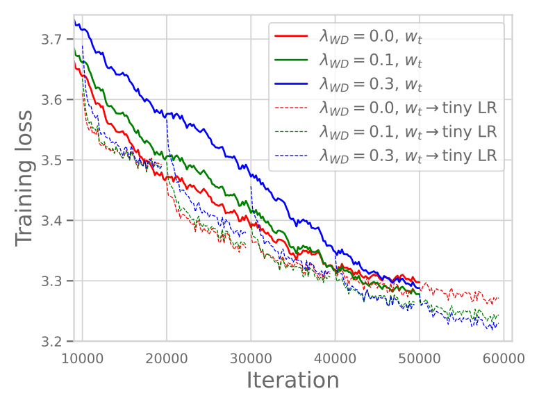
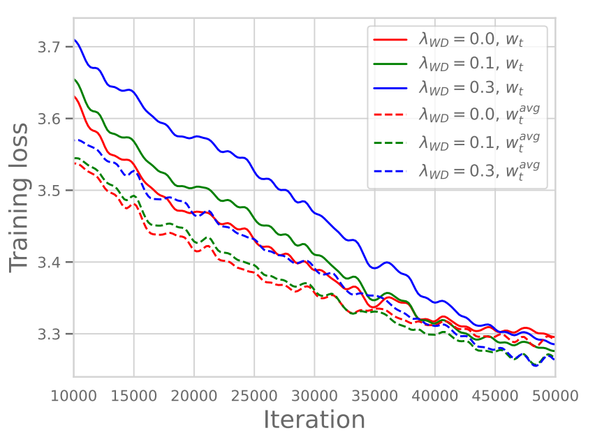
It is precisely from this perspective that the role of WD in the loss term becomes important. Although this has not yet been clearly defined, recent research/papers have revealed a phenomenon, and we can see the results in Figure 1 below. Looking closely at Figure 1, although the Training Loss value might be somewhat larger in the early part of training when strong WD is applied, we can verify that ultimately, it converges to a lower value when larger WD is applied.

In that lecture, Professor Hashimoto interprets this as follows:

(Paraphrased) Due to LR Scheduling, the Learning Rate decreases as it moves toward the latter part of training, and accordingly, the Gradient also decreases. Therefore, the training effect may become insignificant at the very end of training. At this time, if we apply strong WD, it can maintain the Gradient values at a certain magnitude even at the end of training, enabling continuous learning.

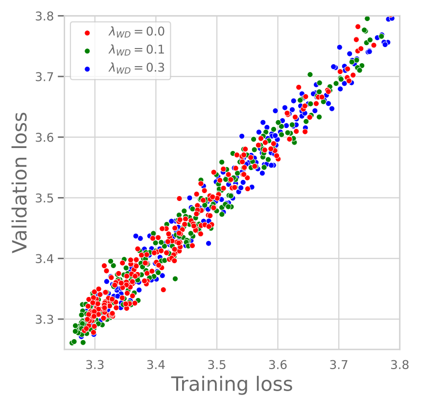
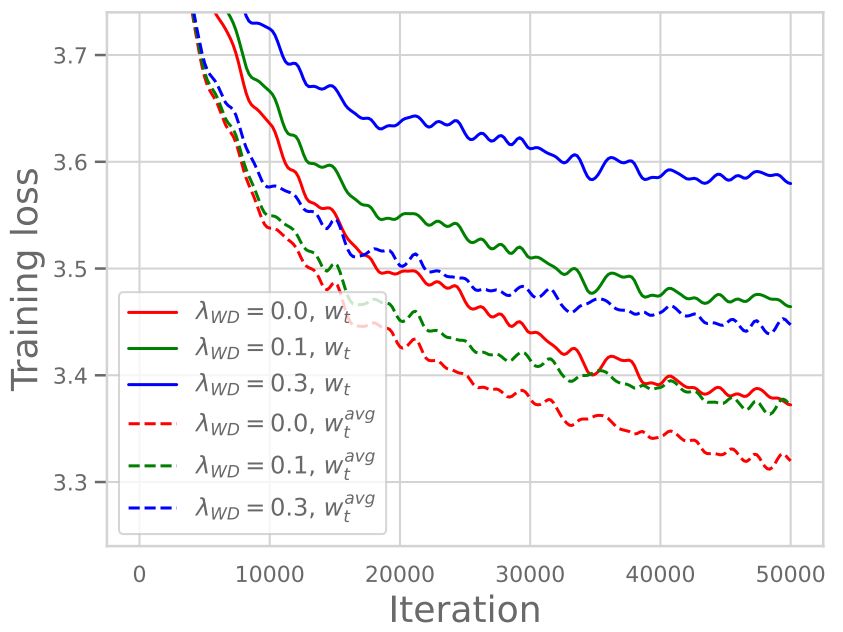
Research results supporting this are also shown in Figure 2 below.

First, the graph on the left shows the relationship between Training & Validation Loss for different WD values. As can be seen in the graph, the Training Loss and Validation Loss values appear almost identical regardless of whether the WD value is large or small. In other words, we can see that the Generalization Gap converges to almost 0 regardless of the WD size. This clearly shows that WD in LLM training is unrelated to preventing Overfitting (Generalization).

On the other hand, the graph on the right shows the results for different WD values when using Constant LR (keeping the Learning Rate constant without decreasing). Here, unlike Figure 1, we can see that the Training Loss value rather increases as WD gets larger. In other words, in a situation where the LR does not decrease, applying strong WD has the effect of strongly constraining the Prior; rather than improving performance, it causes harm to performance.

Synthesizing the contents above, it is helpful to understand that WD in LLMs is used to maintain the continuity of training in conjunction with LR Scheduling, unlike the traditional concept of preventing overfitting.

Conclusion

In conclusion, Weight Decay (WD) can be viewed from two perspectives: the Statistical Perspective and the Optimization Perspective:

• Viewed from the Statistical Perspective, by introducing a Gaussian Prior to the MLE method which relies entirely on data and converting it to MAP estimation, it prevents data bias and allows finding a stable solution.
• At the same time, from the Optimization Perspective, it performs the role of guaranteeing the continuity of training by preserving the magnitude of the Gradient, which decreases as Learning Rate Decay progresses during large-scale training like LLMs.

In other words, WD can be defined as performing two core functions according to the setting: limiting the Hypothesis Space through Prior to search for the optimal solution from a statistical perspective and maintaining training momentum from an optimization perspective.

I have organized concepts used in deep learning after a long time. I will often post about concepts that are used frequently but whose beyond can be examined. Thank you for reading.

Reference

• Bishop, Christopher M. Pattern Recognition and Machine Learning. New York :Springer, 2006. (Original Book)
• Andriushchenko, Maksym, et al. “Why do we need weight decay in modern deep learning?.” ICLR (2023). (Paper)
• Stanford CS336 Lecture 3 (Youtube)