[Conceptual Background] Sharpness-Aware Minimization Through the Lens of Shrinkage Theory

(This post was translated from the original Korean version with the assistance of ChatGPT.)

TL;DR: In this post, I revisit Sharpness-Aware Minimization (SAM) and explore how its geometric behavior can be understood through the lens of Shrinkage Theory.

About Generalization & Robustness in Deep Learning

Recently, generalization and robustness have remained important topics in Deep Learning. One reason is that the amount and quality of available data are rarely ideal. Real-world data are often noisy, and it is not always possible to remove every unwanted variation during preprocessing. Even when a model is trained using carefully prepared data, we cannot necessarily guarantee that the data encountered after deployment will have the same quality or distribution.

For this reason, many approaches have been developed to improve the generalization and robustness of deep learning models. One representative approach is Sharpness-Aware Minimization (SAM) [3]. In this post, I will first revisit how SAM works and then look at it from a slightly different perspective, connecting the geometry of the loss landscape to classical Shrinkage Theory.

Deep Learning Models Are Overparameterized

Before discussing SAM itself, it is helpful to look a little more closely at what it means to train a deep learning model. In general, a model can be represented as a function $f(x;\theta)$, where $\theta\in\mathbb{R}^d$ denotes its trainable parameters. Training means finding a combination of these $d$ parameters that performs well on a given task.

However, there is usually no reason to assume that only one parameter configuration can solve the task. Modern deep learning models are highly overparameterized. Even a relatively familiar model such as ResNet-18 contains approximately 11.7 million parameters. Therefore, a large number of different parameter configurations may achieve similarly low training loss.

At this point, we need to consider overfitting. A model can fit the observed training data very well without necessarily learning a solution that generalizes to unseen data. Studies on overparameterization have also shown that the relationship between model size and generalization is more complicated than the classical intuition might suggest [1][2], as illustrated by phenomena such as double descent.

Still, the general concern remains: a low training loss alone does not guarantee that a model will behave reliably when the data change. In a loose sense, a sufficiently expressive model may learn characteristics that are too specific to its training dataset, including noise that is not useful outside that dataset.

(This is one of the situations in which we commonly discuss overfitting and the limits of generalization.)

Improving Generalization and Robustness

A practical objective is to obtain a model whose predictions do not change excessively under small, relevant variations in the input or environment. There are several ways to approach this problem, but two intuitive directions are:

1. Increase the diversity or amount of training data, for example through additional data collection or Data Augmentation.
2. Change the training procedure so that the resulting model favors solutions that are less sensitive to perturbations.

The first direction exposes the model to more cases during training. The second concerns the properties of the learned solution itself. SAM belongs to this second direction, but with one important distinction: SAM explicitly considers perturbations in parameter space, rather than directly perturbing the input data. Its connection to data robustness and generalization is a motivation and an empirical observation, not an unconditional guarantee.

With this distinction in mind, I will first explain SAM in terms of the loss landscape.

What Is Sharpness-Aware Minimization (SAM)?

Sharp Minima & Flat Minima

As mentioned in the previous section, SAM aims to find solutions with better generalization properties by looking at the geometry of the loss landscape. When training a neural network, we usually monitor the loss value. However, two solutions can have almost the same loss while exhibiting quite different behavior in their surrounding parameter neighborhoods.

Figure 1 illustrates this distinction between sharp minima and flat minima.

(For more details on visualizing neural-network loss landscapes, please refer to [4].)

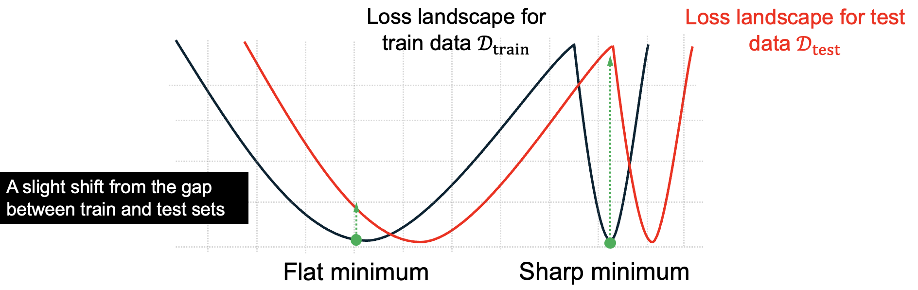
In a sharp minimum, a relatively small change in the parameter values can cause a large increase in loss. In a flat minimum, similar parameter perturbations tend to produce smaller changes in loss. Therefore, even when both solutions have similarly low training loss, their local sensitivity can be quite different.

This leads to the motivation behind SAM: rather than minimizing only the loss at one particular parameter configuration, we can try to find a solution whose loss remains low in its surrounding neighborhood. This is one way to encourage flatter solutions, which are often associated with improved generalization.

Sharpness-Aware Minimization (SAM)

To understand how SAM encourages flatter minima, it helps to compare it with ordinary model training. In conventional gradient-based optimization, we calculate the loss at the current parameters and update the parameters in a direction that reduces that loss.

SAM takes a slightly different approach. It first looks for a nearby parameter perturbation that produces a large loss, and then updates the model to reduce the loss at that perturbed point. In other words, SAM does not focus only on obtaining a low loss at the current parameter values. It also considers how the loss behaves when those values are changed slightly.

The objective can be written as follows:

Here, $\theta$ denotes the model parameters, $\mathcal{L}$ is the loss function, $\epsilon$ is a perturbation applied to the parameters, and $\rho$ is a hyperparameter that determines the maximum perturbation radius. The objective consists of two steps:

• Inner Maximization: Find the perturbation $\epsilon$ within radius $\rho$ that maximizes the loss around the current parameters.
• Outer Minimization: Update the parameters to minimize the loss obtained at the perturbed point.

In other words, SAM repeatedly identifies a direction in which the loss is likely to increase and then updates the model to reduce the loss there. A useful intuitive picture is that it tries to press down the steep parts of the loss landscape rather than simply moving toward a low-loss point.

Now, I will go through how these two steps are computed in practice.

Inner Maximization

As summarized above, Inner Maximization finds a perturbation $\epsilon$ within radius $\rho$ that maximizes the loss around $\theta$. However, checking every possible perturbation one by one is practically impossible. Deep learning models have a very large number of parameters, so searching all directions in the parameter space would require an enormous amount of computation.

Fortunately, we can use one of the most common tools in engineering: approximation. The original SAM method uses a Taylor Expansion to approximate the loss function locally. Starting with the second-order expansion, we obtain:

Here, $H(\theta)=\nabla_{\theta}^{2}\mathcal{L}(\theta)$ denotes the Hessian matrix, which describes local loss curvature. The first-order term explains how the loss changes along a direction, whereas the second-order term describes how that rate of change varies with curvature.

Including the Hessian term in the maximization makes the problem more computationally involved. Explicitly forming a full Hessian is also impractical for modern neural networks, although Hessian-vector products can be computed without constructing the entire matrix. For efficiency, the practical SAM perturbation uses the first-order approximation:

(The original SAM paper also investigates approximations involving higher-order information; the first-order method provides a practical trade-off between computation and performance.)

At this point, the remaining task is to find the worst-case perturbation under the radius constraint. Although $\rho$ determines the allowed neighborhood, the loss does not necessarily increase equally in every direction inside that neighborhood. We therefore need a way to identify the perturbation that maximizes the approximated loss.

The original problem is:

Using the first-order approximation, we instead solve:

The term $\mathcal{L}(\theta)$ disappears from the maximization because it does not depend on $\epsilon$. Therefore, we only need to maximize the inner product between the gradient and the perturbation.

The Cauchy–Schwarz Inequality gives a convenient upper bound:

Since the perturbation norm is constrained by $\rho$, the upper bound is achieved, when the gradient is nonzero, by choosing a perturbation in the same direction as the gradient, with norm $\rho$. Thus, we obtain:

This result is quite simple. We normalize the gradient to preserve its direction and then scale it to the allowed radius $\rho$. In this way, SAM approximates the worst-case perturbation using only one gradient computation, rather than evaluating all possible perturbations.

Of course, this is the maximizer of the first-order approximation, not necessarily the exact maximizer of the original nonlinear loss. The approximation trades some accuracy for computational efficiency, which is one reason why SAM is practical.

Outer Minimization

After obtaining the approximate worst-case perturbation $\hat{\epsilon}$, the next step is to minimize the loss at the perturbed parameter point. This is the Outer Minimization step.

Compared with ordinary model training, the main difference is the location where the gradient is evaluated. In conventional optimization, we calculate the gradient at $\theta$. In SAM, we first apply $\hat{\epsilon}$ and then evaluate the gradient at $\theta+\hat{\epsilon}$.

The resulting surrogate loss can be written as:

There is one detail worth examining here. The perturbation $\hat{\epsilon}$ itself is computed from the gradient at $\theta$, so it also depends on $\theta$. If we differentiate the full expression through this approximate perturbation, the chain rule introduces additional terms that involve second-order derivatives.

In practice, SAM treats the computed perturbation as fixed when taking the outer gradient, avoiding those additional computations. When the inner maximization is solved exactly under suitable regularity conditions, the envelope-theorem viewpoint also explains why the derivative through the maximizer is not needed. In practical SAM, however, the inner maximizer is only approximated, so the resulting gradient is also an approximation.

Therefore, instead of explicitly calculating the Hessian in the outer step, we calculate another gradient at the perturbed point. Using learning rate $\eta$, the parameter update becomes:

The important point is that the gradient is evaluated at $\theta_t+\hat{\epsilon}_t$, but the update is applied to the original parameters $\theta_t$. Conceptually, SAM temporarily probes the surrounding high-loss direction, obtains a gradient there, and then uses that gradient to update the current model.

Putting the two steps together, SAM finds a direction in which the loss is likely to increase and trains against that direction. This encourages solutions with lower loss sensitivity within the neighborhood. The main computational drawback is that one gradient is needed for the inner step and another for the outer step, giving approximately twice the usual gradient-evaluation cost.

Recap of SAM

To summarize the mechanism of SAM once again:

• Objective: Encourage solutions with lower worst-case loss in a parameter neighborhood, often associated with flatter minima and improved generalization.
• Training procedure:

  1. Gradient and perturbation: Compute the gradient at $\theta_t$ and approximate the worst-case perturbation.

     \[\hat{\epsilon}_t=\rho\frac{\nabla_{\theta}\mathcal{L}(\theta_t)}{\|\nabla_{\theta}\mathcal{L}(\theta_t)\|_2}\]

  2. Perturbed gradient: Evaluate the gradient at the perturbed point $\phi=\theta_t+\hat{\epsilon}_t$.

     \[\nabla_{\phi}\mathcal{L}(\phi)\big|_{\phi=\theta_t+\hat{\epsilon}_t}\]

  3. Parameter update: Update the original parameters using the perturbed gradient.

     \[\theta_{t+1}=\theta_t-\eta\nabla_{\phi}\mathcal{L}(\phi)\big|_{\phi=\theta_t+\hat{\epsilon}_t}\]
• Main intuition: Find a direction in which the loss becomes large, then update the model to reduce the loss at that point.
• Computational limitation: Two gradient evaluations are required, approximately doubling the corresponding computation relative to ordinary SGD.

Many variants of SAM have been proposed to address its limitations or modify the way sharpness is handled. Some representative examples are:

• Adaptive SAM (ASAM) [5]: Adjusts the perturbation geometry according to parameter scale, addressing the sensitivity of ordinary SAM sharpness to parameter rescaling.
• Surrogate Gap SAM (GSAM) [6]: Introduces a surrogate gap and seeks to reduce it in addition to the perturbed loss, encouraging improved flatness.
• Efficient SAM (ESAM) [7]: Reduces training cost by using selective weight perturbations and choosing data samples that are more informative for sharpness-aware training.
• Bayesian SAM (BayesianSAM) [8]: Connects SAM to a Bayesian interpretation and introduces a probabilistic perspective on sharpness-aware optimization.
• LookSAM [9]: Reuses information from previously computed SAM updates to reduce how frequently the full SAM computation is needed.

After SAM was introduced, research expanded in several directions, including finding flatter solutions more effectively and reducing computational overhead. More recently, there has also been interest in understanding what happens when flatness-aware learning is applied beyond ordinary supervised learning. For example, research from our lab has examined flatness in Reinforcement Learning [10] and Generative Models [11]. Related questions continue to appear in many other learning settings.

Linking SAM to Shrinkage Theory

While working on SAM-related research, I had an opportunity to discuss it with one of the leading authorities in the field. After looking at SAM, the researcher casually commented that “This looks quite similar to shrinkage methods.” I did not immediately see the connection, but after thinking about the comment and discussing it further, including some conversations with an LLM, I started to see an interesting geometric similarity between the two ideas.

The connection may not be strong enough by itself to constitute a new research contribution. Still, I thought it would be interesting to organize the intuition in a blog post. The goal here is not to argue that SAM and Shrinkage Theory are mathematically equivalent, but to explore a common perspective through the eigen-spectrum of a matrix.

(Muon also started as a blog discussion before becoming a broader research topic. Perhaps this connection could lead to something interesting in the future as well…!!)

SAM from a Hessian Perspective

So far, I have explained SAM mainly through its optimization procedure. However, when looking at the method from a slightly different perspective, much of the discussion comes back to basic concepts from Machine Learning: convexity and loss curvature. A central object in understanding this local geometry is the Hessian.

As discussed above, practical SAM does not explicitly compute the Hessian for its parameter update. Nevertheless, since SAM seeks solutions with lower loss sensitivity in a local neighborhood, the Hessian provides a useful way to understand the curvature properties associated with such solutions.

(There are also related approaches such as FisherSAM, which consider the geometry of parameter perturbations using the Fisher Information Matrix (FIM). The FIM is related to, but is not generally identical to, the loss Hessian.)

I will begin with the second-order Taylor expansion introduced earlier:

To make the geometric interpretation clearer, suppose that the parameters $\theta^{\ast}$ lie at a differentiable local minimum. At that point, the gradient vanishes:

The first-order term therefore disappears, leaving the second-order approximation:

In other words, the local increase in loss around a minimum is determined, to second order, by the Hessian. This is where the eigenvalues become important.

Because the Hessian of a twice continuously differentiable scalar loss is a symmetric matrix, it admits an eigendecomposition:

Here, $Q$ contains the eigenvectors and $\Lambda$ contains the corresponding eigenvalues. Each eigenvector represents a direction in parameter space, and its eigenvalue describes the curvature of the loss in that direction. Around a local minimum, nonnegative eigenvalues describe how quickly the loss rises along the corresponding directions.

A large eigenvalue indicates a direction with relatively high curvature, whereas a small eigenvalue indicates a comparatively flat direction. The geometric interpretation becomes especially clear when we look at a two-dimensional example.

Suppose the two Hessian eigenvalues are $\lambda_1=10$ and $\lambda_2=1$. Since the curvature along the first direction is much larger, the same displacement leads to a much greater increase in loss along that direction. As a result, contours of equal loss form an elongated elliptical shape. By contrast, if $\lambda_1=\lambda_2=1$, the curvatures are identical and the corresponding quadratic contours become circles, or isotropic contours in two dimensions.

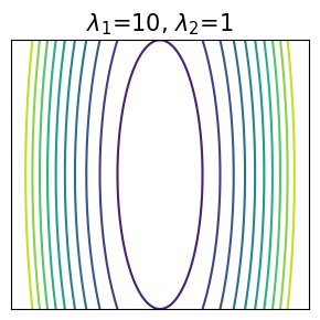
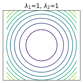
This distinction is important because flatness and isotropy are not the same thing. Flatness concerns the magnitude of curvature, whereas isotropy concerns how similar the curvatures are across different directions. It is possible to reduce all eigenvalues by the same factor and obtain a flatter landscape without making its contours more circular.

Now, I will connect this Hessian perspective back to SAM. Applying the second-order approximation to its inner maximization at $\theta^{\ast}$ gives:

The key point is that the increase in loss depends on the direction of $\epsilon$. Since the eigenvectors of the Hessian form an orthonormal basis, we can express any perturbation in that basis:

Here, $q_i$ is the $i$-th eigenvector and $a_i$ represents the size of the perturbation along that direction. Substituting this expression into the quadratic term gives:

Therefore, the quadratic increase in loss is determined by the eigenvalue of each direction and how much perturbation is allocated to that direction. However, SAM does not allow the perturbation magnitude to grow without limit. Its radius constraint becomes:

Under this constraint, concentrating the perturbation along a direction with a larger eigenvalue produces a larger quadratic loss increase. In particular, the following upper bound holds:

Here, $\lambda_{\max}(H)$ is the maximum Hessian eigenvalue. At a twice-differentiable local minimum, the Hessian is Positive Semi-Definite (PSD). Thus, the upper bound is attained by a perturbation of length $\rho$ along a maximum-eigenvalue direction, provided the maximum eigenvalue is positive. This gives the familiar local quadratic interpretation of the SAM objective:

This relation captures an important property of SAM. From a second-order perspective near a local minimum, a solution with a large maximum Hessian eigenvalue receives a larger worst-case-neighborhood loss penalty. Consequently, when comparing otherwise similar low-loss solutions, SAM tends to favor those with smaller dominant curvature.

It is important to keep the scope of this statement in mind. This is a local quadratic interpretation of the worst-case objective, not a statement that the practical first-order SAM algorithm explicitly computes or necessarily decreases the maximum eigenvalue at every iteration.

Still, this viewpoint suggests an interesting geometric observation. If an excessively large curvature direction becomes less dominant, an elongated loss contour can become less anisotropic. A related operation appears in statistics, where extreme eigenvalues can be pulled toward a common target. This brings us to Shrinkage Theory.

What Is Shrinkage Theory?

Shrinkage Theory

Shrinkage Theory is a concept developed in statistics. In simple terms, it describes the idea of moving an estimate toward a chosen target in order to improve estimation accuracy.

In statistical modeling, we often estimate unknown parameters from observed data. However, real-world datasets contain noise, and the number of available samples is not always sufficient. Therefore, even when we use a reasonable estimation procedure, the estimated parameter can differ from its true value.

One way to address this issue is to adjust the estimate we already have, rather than relying entirely on the observed data. This is the basic intuition behind Shrinkage. A simple shrinkage estimator can be written as:

Here, $\hat{\theta}$ is the estimate obtained from data, $\theta_0$ is the shrinkage target, and $\alpha\in[0,1]$ is the coefficient controlling the strength of shrinkage. The target determines the reference value toward which the estimate is adjusted. Depending on the problem, it may be chosen from prior knowledge, a population mean, or another stable reference estimate.

When $\alpha=0$, we keep the original estimate. When $\alpha=1$, we use the target directly. For intermediate values, we combine the two.

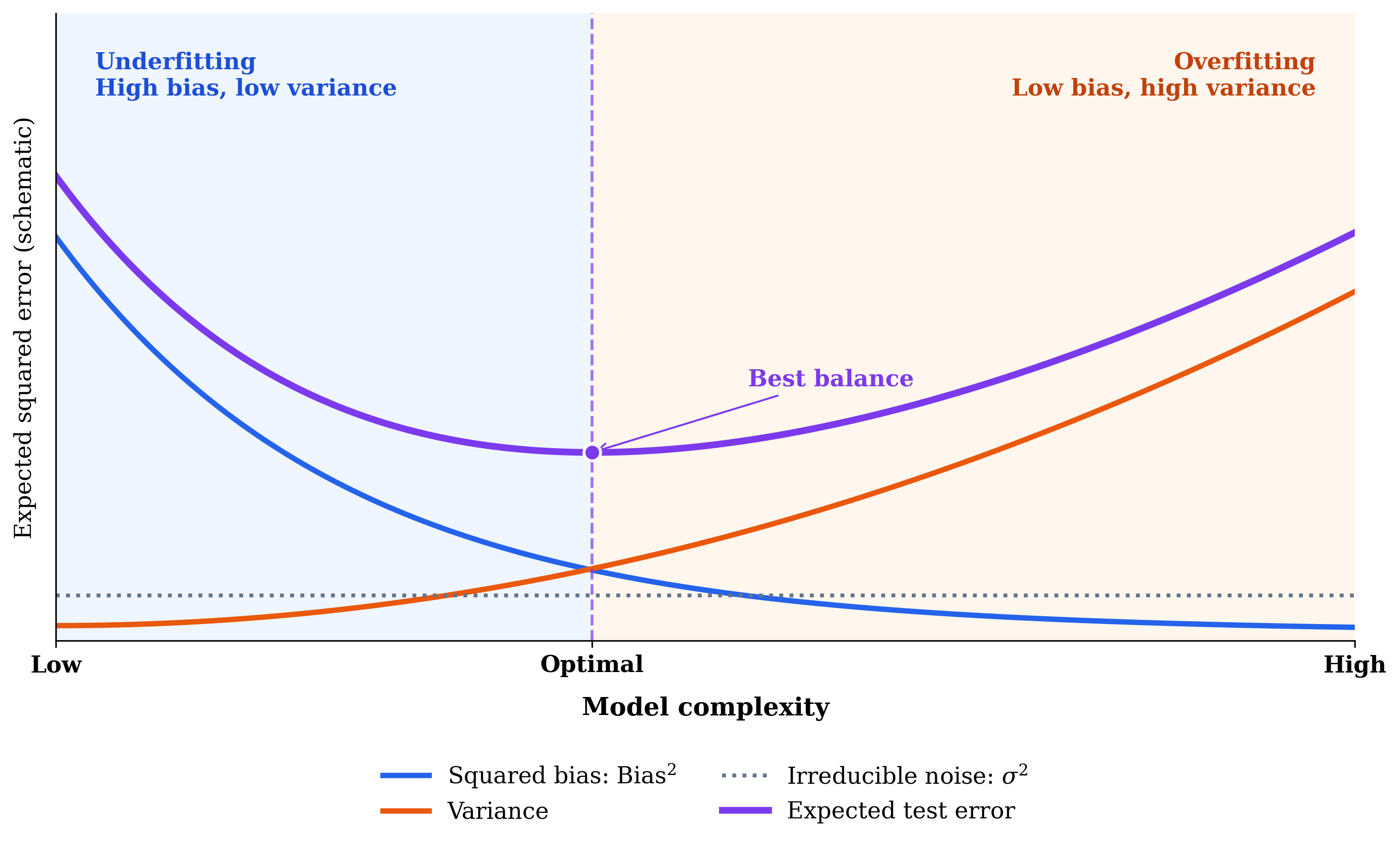
At first, moving an estimate away from the value obtained from data may seem counterintuitive. However, this is exactly where the statistical Bias–Variance Tradeoff becomes important [12]. The Mean Squared Error (MSE) of a scalar estimator can be decomposed as:

Here, Bias measures how far the estimator’s expected value is from the true parameter, whereas Variance describes how much the estimator changes across repeated samples. Therefore, estimation accuracy depends not only on whether an estimator is centered at the true value, but also on how stable it is when the observed data change.

Figure 3 illustrates the familiar intuition behind the Bias–Variance Tradeoff.

To connect this with shrinkage, I will use a simple scalar example. Let the true parameter be $\theta$ and assume that our original estimator $\hat{\theta}$ is unbiased:

We now apply the shrinkage transformation introduced above:

For simplicity, assume that both $\alpha$ and $\theta_0$ are fixed rather than estimated from the same random sample. Taking the expectation yields:

The resulting bias is therefore:

Although the original estimator had zero bias, shrinkage generally introduces bias proportional to the distance between the target and the true parameter. This may initially look like a disadvantage. However, the variance behaves differently:

Since $\alpha\in[0,1]$, we have $(1-\alpha)^2\leq1$. In other words, the variance of this shrinkage estimator cannot exceed the variance of the original estimator under the fixed-target assumption.

Combining the two results gives:

This equation summarizes the main idea. Shrinkage can introduce bias while reducing variance, and the overall MSE becomes smaller when the variance reduction outweighs the increase in squared bias.

For example, suppose the true parameter is $\theta=3$, the original estimator is unbiased with variance $4$, and we choose $\theta_0=2$ and $\alpha=0.5$. The original and shrunk MSE values are:

In this case, introducing bias actually improves the total estimation error because the decrease in variance is larger. Of course, shrinkage is not automatically better for every target or every coefficient. A poorly chosen target or excessive shrinkage can increase the MSE instead.

A classical example of the statistical value of shrinkage is the James–Stein estimator [13], which demonstrates that shrinking a multivariate Gaussian mean estimator can reduce the overall squared-error risk under suitable conditions.

Now, I will return to the original purpose of this post. The connection we are interested in is not simply parameter estimation, but the eigenvalues of the Hessian that appeared in our analysis of SAM. Although ordinary shrinkage does not directly involve Hessian eigenvalues, a closely related example does involve matrix eigenvalues: Covariance Shrinkage.

Covariance Shrinkage

Covariance Shrinkage applies the shrinkage idea to a covariance matrix. A covariance matrix describes how variables vary together and how data are dispersed along different directions. Like the Hessian, it is symmetric, and its eigenvalues and eigenvectors provide a geometric interpretation of the corresponding directions.

In practice, the true covariance of a data distribution is usually unknown. We therefore estimate it from observed samples, obtaining a Sample Covariance Matrix $S$. As with other estimators, a sample covariance matrix can contain estimation error. This becomes particularly problematic when the dimension is large relative to the sample size, because the sample eigenvalues can be poorly estimated and the resulting matrix can become ill-conditioned or even singular.

One way to improve the stability of this estimate is to shrink the sample covariance matrix toward a chosen target matrix. A representative approach is the covariance shrinkage estimator studied by Ledoit and Wolf [14]:

Here, $S$ denotes the sample covariance matrix, $I$ is the identity matrix, and $\mu$ determines the scale of the target matrix. One common choice is $\mu=\mathrm{tr}(S)/d$, the average eigenvalue of $S$.

This expression is almost identical in structure to the scalar shrinkage estimator introduced earlier. The difference is that we now adjust an entire matrix toward a target matrix, rather than adjusting a single estimate toward a scalar target.

There is one particularly interesting property here: this matrix-level shrinkage can also be understood directly in terms of eigenvalues.

As with the Hessian, the sample covariance matrix admits an eigendecomposition:

Substituting this decomposition into the shrinkage formula gives:

The key observation is that the original eigenvector basis can be preserved. Since $Q$ is an orthogonal matrix, $Q^\top Q=I$, and the isotropic target can be represented in the same basis:

In other words, both the original covariance matrix and its target $\mu I$ can be expressed using the same eigenvector basis. As a result, this particular shrinkage transformation leaves that eigenvector basis unchanged and modifies only the eigenvalues.

Each original eigenvalue $\lambda_i$ is transformed into:

This is the central equation for the geometric interpretation of covariance shrinkage. Every eigenvalue is pulled toward the common target $\mu$. Eigenvalues above $\mu$ decrease, while those below $\mu$ increase. Consequently, the differences among eigenvalues become smaller:

Thus, for $0\leq\alpha\leq1$, the spectral spread is contracted by a factor of $(1-\alpha)$. In the geometric picture introduced in Figure 2, this resembles the process of making an anisotropic, elongated ellipse more isotropic. For a positive-definite covariance matrix, the level-set geometry becomes less elongated as the eigenvalue ratios become more similar.

Here, I want to focus on one more quantity: the Maximum Eigenvalue. When $\mu$ is chosen as the mean eigenvalue, $\lambda_{\max}\geq\mu$. After shrinkage, the excess of the maximum eigenvalue above the target changes as follows:

That is, the maximum eigenvalue is pulled closer to the mean as the overall spectrum becomes more uniform. This is the specific geometric behavior that reminded me of the Hessian interpretation of SAM.

Of course, the original goal of Covariance Shrinkage is to improve the accuracy and numerical stability of a noisy covariance estimate, not to manipulate a neural network’s loss Hessian. Nevertheless, the resulting Spectral Contraction gives us a useful common language for comparing shrinkage with sharpness-aware optimization.

Returning to SAM, the local second-order analysis showed that its worst-case neighborhood loss is related to $\lambda_{\max}(H)$. Accordingly, SAM favors solutions with lower dominant curvature when comparing otherwise similar local minima. In Covariance Shrinkage, the large eigenvalues of an estimated matrix are explicitly moved toward a target.

Both perspectives therefore place special emphasis on excessive spectral components, although they act on different mathematical objects and use different mechanisms. Covariance Shrinkage directly transforms matrix eigenvalues, whereas SAM optimizes a worst-case loss and may favor a solution with smaller dominant Hessian curvature.

It would be too strong to claim that “SAM and Shrinkage are the same method.” SAM does not explicitly shrink each Hessian eigenvalue toward its mean, nor does it guarantee that a learned minimum becomes isotropic. But the suppression of dominant curvature provides a geometric analogy that can be useful for interpreting what SAM encourages during optimization.

Conclusion

Wrap-Up

(Almost done!!)

In this post, I revisited Sharpness-Aware Minimization (SAM) from the perspective of Hessian curvature and tried to connect it with the spectral interpretation of Shrinkage Theory.

First, near a twice-differentiable local minimum, the worst-case quadratic loss increase in a parameter neighborhood can be written in terms of the maximum Hessian eigenvalue:

On the other hand, Shrinkage Theory adjusts an estimate toward a target to balance bias and variance. If we hypothetically apply the isotropic spectral transformation used in Covariance Shrinkage to a Hessian, we obtain:

Here, $\mu$ is the mean Hessian eigenvalue. Since this transformation pulls the maximum eigenvalue toward $\mu$, the associated worst-case quadratic curvature satisfies:

The meaning of this equation is straightforward. Under this hypothetical shrinkage transformation, the worst-case quadratic curvature above the mean is contracted by a factor of $(1-\alpha)$. In this sense, the Spectral Contraction of covariance shrinkage can be expressed using the same maximum-curvature quantity that appears in the local analysis of SAM.

One distinction is essential: the boxed equation does not describe the actual training dynamics of SAM. It describes what happens if the shrinkage transformation is applied to the Hessian. SAM and Covariance Shrinkage do not perform the same operation. In particular, SAM does not guarantee a contraction of the entire Hessian spectrum or an isotropic loss landscape.

Nevertheless, the two methods can be connected through a common geometric perspective: controlling excessively large spectral components. SAM can therefore be interpreted, cautiously, as encouraging an effect resembling implicit shrinkage of dominant curvature, rather than literally carrying out a covariance-shrinkage transformation.

That is the main point I wanted to share: SAM and Shrinkage Theory start from different perspectives, but the eigen-spectrum provides a useful geometric connection between them.

Final Remarks

It has been a while since I wrote a long conceptual post, and the explanation ended up being longer than I originally planned. I wanted to preserve the intuition while also showing the mathematical steps behind it. I will continue refining the post as I revisit the ideas and related literature. If there are errors in the explanation or other perspectives worth considering, I would be happy to hear them and incorporate the feedback. 😀😀

Thank you for reading this long post!!

Reference

[1] Zhang, Chiyuan, et al. “Understanding Deep Learning Requires Rethinking Generalization.” ICLR (2017). (Paper)

[2] Nakkiran, Preetum, et al. “Deep Double Descent: Where Bigger Models and More Data Hurt.” ICLR (2020). (Paper)

[3] Foret, Pierre, et al. “Sharpness-Aware Minimization for Efficiently Improving Generalization.” ICLR (2021). (Paper)

[4] Li, Hao, et al. “Visualizing the Loss Landscape of Neural Nets.” NeurIPS (2018). (Paper)

[5] Kwon, Jungmin, et al. “ASAM: Adaptive Sharpness-Aware Minimization for Scale-Invariant Learning of Deep Neural Networks.” ICML (2021). (Paper)

[6] Zhuang, Juntang, et al. “Surrogate Gap Minimization Improves Sharpness-Aware Training.” ICLR (2022). (Paper)

[7] Du, Jiawei, et al. “Efficient Sharpness-Aware Minimization for Improved Training of Neural Networks.” ICLR (2022). (Paper)

[8] Möllenhoff, Thomas, and Mohammad Emtiyaz Khan. “SAM as an Optimal Relaxation of Bayes.” ICLR (2023). (Paper)

[9] Liu, Yong, et al. “Towards Efficient and Scalable Sharpness-Aware Minimization.” CVPR (2022). (Paper)

[10] Lee, Hyun Kyu, and Sung Whan Yoon. “Flat Reward in Policy Parameter Space Implies Robust Reinforcement Learning.” ICLR (2025). (Paper)

[11] Lee, Taehwan, et al. “Understanding Flatness in Generative Models: Its Role and Benefits.” ICCV (2025). (Paper)

[12] Geman, Stuart, Elie Bienenstock, and René Doursat. “Neural Networks and the Bias/Variance Dilemma.” Neural Computation 4(1) (1992). (Paper)

[13] James, William, and Charles Stein. “Estimation with Quadratic Loss.” Proceedings of the Fourth Berkeley Symposium on Mathematical Statistics and Probability (1961). (Source link from original post)

[14] Ledoit, Olivier, and Michael Wolf. “A Well-Conditioned Estimator for Large-Dimensional Covariance Matrices.” Journal of Multivariate Analysis (2004). (Paper)