Denoising Diffusion Probabilistic Model

(간략한) Generative Model들 review

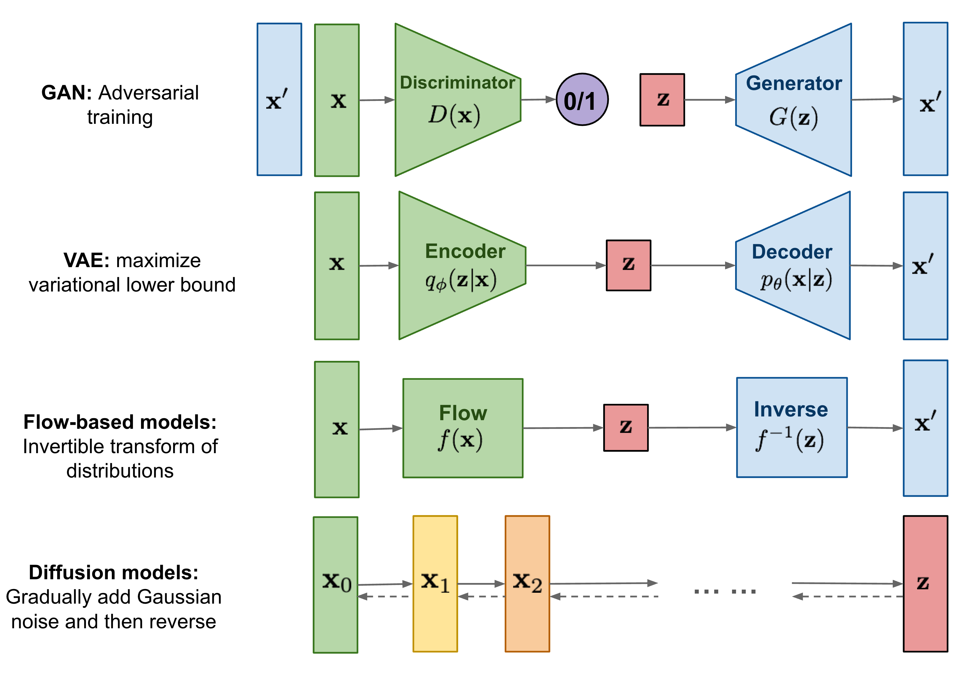
• GAN: Discriminator 와 Generator를 서로 경쟁시켜(adversarial) 학습
• VAE: Input을 Latent space $Z$에 mapping 시킨 후(encoding), latent space로부터 다시 복원(Decoding)
• Flow-based Models: $f(x)$ 함수를 통해 input을 space $Z$ 에 mapping 시킨 후 $f(x)$를 inverse시켜 복원 (iterative)
• Diffusion Model: Gaussian Noise를 점진적으로 추가하여 high entropy 상태에서 과정을 다시 reverse함을 통해 복원 (iterative)

Generative Model의 최종 목적:
$\Rightarrow$ 수학적으로 정의된 distribution (e.g., Gaussian Distribution)으로부터, 즉 정의하기 쉬운 distribution으로부터 특정 pattern을 갖는 distribution 형태로 mapping

Denoising Diffusion (Probabilistic) Model

Diffusion Model Method:

• 기본적으로 parameterized Markov Chain 형태의 model 형태로 존재 (Sequential 한 형태)
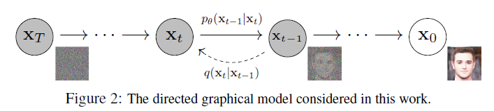
• 원본 data $X_0$ 에 매 step마다 Gaussian Noise를 추가하여 high entropy 상태의 data $X_T$ 로 변환 (diffusion; forward process)
  $\rightarrow$ $T = \infty $ 일 경우 data $X_T$ 는 data $X_0$ 의 특징(feature)를 완전히 잃음
• High Entropy 상태의 data $X_T$ 를 원본 data $X_0$로 복원 (Reverse Process)

Diffusion Model Process:

Forward Process :
\(q(X_{1:T} | X_0) = \prod_{t=1}^{T} q(X_t |x_{t-1} ), \; q(X_t | X_{t-1}) = \mathcal{N}(X_t ; \sqrt{1-\beta_t}X_{t-1} , \beta_t I) \tag{1}\)

Reverse Process : \(p_{\theta}(X_{0:T}) = p(X_T) \prod_{t=1}^T p_{\theta}(X_{t-1}|X_T), \; p_\theta(X_{t-1}|X_t) = \mathcal{N}(X_{t-1} ; \mu_\theta (X_t, t) , \Sigma_\theta(X_t, t)) \tag{2}\)

• $p$는 학습시켜야 하는 model, $q$는 fixed (Gaussian Noise)
  $\rightarrow$ 기존 diffusion model에서는 $\beta_t$도 학습을 통해 도출했으나, experimentally 확인 결과 fixed value여도 큰 차이가 없다고 합니다.
• $\beta_t$ 가 작으면 작을수록 $X_t$의 변화율 $\downarrow$
  $\Rightarrow$ Gaussian Noise의 variance 값이 $\downarrow$ & mean 값의 변화율 $\downarrow$
• Reverse Process에서 $p_\theta(X_{t-1}|X_T)$ $\Rightarrow$ 학습을 통해 mean & variance를 예측하는 방향으로 update
• Forward Process의 $q$가 Gaussian을 따르기 때문에 Reverse Process에서 $p_\theta$도 Gaussian을 따릅니다. $\Rightarrow$ 증명: Feller, 1949

Diffusion Loss

VAE Loss:

\[\color{red}{D_{KL} (q_\phi (z|x)||p_\theta(z))} \color{black}+\color{blue}{\mathbb{E}_{q_\phi (z|x)}[\log p_\theta (z|x)]} \tag{3} \Rightarrow \color{red}{\text{Regularization}} \color{black}+ \color{blue}{\text{Reconstruction}}\]

Diffusion Loss:

\[\begin{align} &\color{red}{\mathbb{E}_q [D_{KL}(q(X_T|X_0)||p(X_T))} \color{black}{+} \color{blue}{\sum_{t>1} D_{KL}(q(X_{t-1}|X_t , X_0)||p_{\theta} (X_{t-1}|X_t)) - \log p_\theta(X_0 | X_1)]} \tag{4} \end{align}\]

• Regularization : learning $\beta_t$
• Reconstruction : Noise 제거 및 기존 data 복원

  • $q (X_{t-1} | X_t , X_0)$ : Diffusion Process의 reverse process 설명

    \[q(X_{t-1}|X_t , X_0) = \mathcal{N}(X_{t-1}; \tilde{\mu}(X_{t-1}, X_0), \beta_t I)) \tag{4-1}\]

  • $X_0$ 의 역할: 이미 $X_0$를 알고 있으니 $q(X_t|X_{t-1})$ 를 Bayesian 으로 풀면 $X_{t-1} \leftarrow X_t$ 정의 가능

    \[\tilde{\mu}(X_{t-1}|X_0) = \frac{\sqrt{\tilde{\alpha}_{t-1}} \cdot \beta_t}{1-\tilde{\alpha}_t}X_0 +\frac{\sqrt{\tilde{\alpha}_{t}} \cdot (1-\tilde{\alpha}_{t-1})}{1-\tilde{\alpha}_t}X_t \tag{5}\]

    where $\tilde{\beta}_t = \frac{1-\tilde{\alpha}_{t-1}} {1 - \tilde{\alpha}_t} \beta_t$ , $\alpha_t = 1- \beta_t$ , $\tilde{\alpha}_t = \prod_{s=1}^{t} \alpha_t $

  • $p_\theta (X_{t-1} | X_t)$ : 실제 noise를 보고 reverse process 예측(학습)

*Bayes Rule: $q(X_{t-1}|X_t,X_0) = q(X_t|X_{t-1}, X_0) \frac{q(X_{t-1}|X_t)}{q(X_t | X_0)}$

*Reparameterization:

\[\begin{aligned} X_t &= \sqrt{\alpha_t}X_{t-1} + \sqrt{1-\alpha_t}\epsilon_{t-1}\\ &= \sqrt{\alpha_t \alpha_{t-1}}X_{t-2} + \sqrt{1-\alpha_t \alpha_{t-1}}\bar{\epsilon}_{t-2} \\ &=\cdots \\ &= \sqrt{\bar{\alpha_t}}X_0 + \sqrt{1-\bar{\alpha}_t}\epsilon \end{aligned} \tag{6}\]

where $\epsilon_{t-1} = \mathcal{N}(0, I)$ , $\bar{\epsilon}_{t-t’} = \mathcal{N} (0, (\sum_{t=1}^{t’} \sigma^2_{t’}) I)\;$ and $\; \bar{\alpha}_t = \prod_{t=1}^t \alpha_i$

여기서 $X_t$를 $X_0$ 에 대한 식으로 치환하면

\[X_0 = \frac{1}{\sqrt{\bar{\alpha}_t}}(X_t - \sqrt{1-\bar{\alpha}_t}\epsilon_t)\tag{7}\]

$X_t$와 $X_0$를 $(5)$ 식에 대입하면

\[\tilde{\mu}_t (X_t, X_0) = \frac{1}{\sqrt{\alpha_t}}(X_t - \frac{1-\alpha_t}{\sqrt{1-\bar{\alpha}_t}}\epsilon_t) \tag{8}\]

$\therefore$ $(6)$을 활용하여 reparameterization 진행 후 $\tilde{\mu}_t$를 $X_t$ 와 $\epsilon_t$ 식으로 치환 가능

Denoising Diffusion Probabilistic Model (DDPM)

Loss Simplification: Only Reconstruction term ($\Rightarrow$ Inductive Bias $\uparrow$)

• Use fixed $\beta_t$ (not to learn $\beta_t$) $\rightarrow$ Delete Regularization term

• Not to learn Variance
  $\rightarrow$ $\Sigma_{\theta} (X_t, t) = \sigma^2_t I$ ; $\sigma^2_t = \tilde{\beta}_t = \frac{1-\tilde{\alpha}_{t-1}} {1-\tilde{\alpha}_t} \beta_t $ or $\sigma^2_t = \beta_t$

• Train $\mu_\theta(X_t , t) \rightarrow$ $X_{t-1}$ 의 gaussian mean을 예측, 즉 $t$ 시점에서 $t-1$ 시점일 때의 mean을 예측하기 위한 $\mu_\theta$를 학습 $\Rightarrow p_\theta(X_{t-1}|X_t) = \mathcal{N}(X_{t-1} ; \mu_\theta (X_t, t) , \Sigma_\theta(X_t, t))$ 을 학습한다고 했을 때 위에서 언급한 것 처럼 variance($\Sigma_\theta$)는 고정을 하고 gaussian distribution을 따르므로 mean에 해당하는 $\mu_\theta $만 estimate 하면 됨

다시 정리하면,

• Diffusion Loss에서의 reconstruction term을 보면 최종적으로 parameterize 및 train 시켜야 하는 variable은 $p_\theta$

• $p_\theta$를 학습 시 해당 variable이 gaussian distribution을 따르므로 mean and variance을 학습시키면 됨

• 다만, DDPM에서는 variance를 fixed term으로 두고 학습을 하므로 $\mu_\theta$만 학습시키면 됨

• Diffusion Model에서는 $(4-1), (5), (8)$ 식들을 적용해 $\tilde{\mu_t}$를 estimate 하면 됨 $\rightarrow$ $\tilde{\mu}_t$를 $\mu_{\theta}$ 로 치환하면 다음과 같은 식으로 바꿀 수 있음

  \[\mu_\theta(X_t, t) = \frac{1}{\sqrt{\alpha_t}} (X_t - \frac{1-\alpha_t}{\sqrt{1-\bar{\alpha}_t}}\epsilon_\theta (X_t, t) ) \tag{9}\]

  $\Rightarrow \epsilon_\theta (X_t, t)$는 t 시점에서의 parameterized gaussian distribution (noise)

Diffusion Model에서의  reconstruction loss term만 보면 결국 $q(X_{t-1}|X_t , X_0)$ & $p_\theta (X_{t-1}|X_t)$ 의 차이를 줄이는 쪽으로 학습 진행

$\Rightarrow$ 여기서 $q$ 와 $p_\theta$ 모두 gaussian distribution이고 variance는 fixed value이므로 서로간의 $\mu$ 차이를 줄이는 쪽으로 학습 진행

$\Rightarrow$ 즉, $\mathbb{E}[(8) - (9)]$ 으로 식을 치환해도 무방

$\therefore$ 이를 전개 및 simplify 하면 다음과 같은 식이 도출

\[\begin{align} L_{t-1} &= \mathbb{E}_q[\frac{1}{2\sigma^2_t}||\tilde{\mu}_t (X_t, X_0) - \mu_\theta (X_t, t)||^2] + C\\ \Rightarrow L_{simple}(\theta)&= \mathbb{E}_{t, x_0, \epsilon} [||\epsilon_t - \epsilon_\theta (\sqrt{\tilde{\alpha}_t}X_0 + \sqrt{1-\tilde{\alpha}_t}\epsilon , t )||^2] \tag{10} \end{align}\]

(이 과정이 denoising 과정이기 떄문에 논문에서 denoising이 붙음)

Conclusion

사실상 거의 처음으로 제대로 읽어본 생성모델이였는데 상당히 흥미로웠습니다. 특히, 단순히 학습에 맡기는 것이 아닌 수학적으로 잘 정의함과 동시에 이 잘 정의된 수학을 공학적으로 잘 활용했다는 느낌을 받았습니다. 실은 순수 수학을 이 세상 속에 적용하기는 매우 어렵지만 이를 approximate, 즉 공학적으로 풀어냈을 때 우리에게 굉장히 실용적이게 되고, 이 Diffusion Model, DDPM 등의 논문이 잘 보여준 것 같습니다.

다음 논문으로는 DDPM 다음으로 나온 Denoising Diffusion Implicit Model (DDIM) 논문을 리뷰해볼까 합니다. 매우 부족하지만 끝까지 읽어주셔서 감사합니다!!

Reference:

• Denoising Diffusion Probabilistic Model(DDPM) Paper
• Diffusion Model 수학이 포함된 tutorial
• Lil’Log’s blog - What are Diffusion Models?
• PR-409 Denoising Diffusion Probabilistic Models