[개념설명] Meta Learning (2) - Approaches

2. Meta Learning Apporaches

사실, 이전 post에서 few-shot learning을 설명한 이유는 meta learning을 설명하기 위해서였습니다. Few-shot learning의 개념을 활용하여 다양하게 approach를 적용하는게 meta learning이라고 이해하시면 됩니다. 그럼 거두절미하고 meta learning에는 어떤 개념들이 있는지 보겠습니다.

Meta learning은 기본적으로 다음과 같이 크게 3가지로 분류할 수 있습니다.

• Optimization-based Approach
• Metric-based Approach
• Model-based Approach

각 approach들에 대해서 중요 논문들의 핵심 approach 위주로 설명드리겠습니다. 다만, 여기서는 model-based approach는 skip하겠습니다. model-based approach는 보통 RL에서 많이 쓰이기 때문에 다음에 기회가 된다면 따로 posting 하도록 하겠습니다!!

$S$ 와 $Q$를 어떻게 학습에 활용하는지를 체크하면서 보시면 좋을 것 같습니다.

2.1 Optimization-based Meta Learning

Optimization-based meta learning은 gradient를 중심으로 학습하는 방법입니다. 이에 따라 제일 먼저 언급되는 논문은 바로 2017년에 나온 Model-Agnostic Meta-Learning (MAML) 입니다. 사실상 “Meta Learning”이라는 개념을 대중화시킨 논문이죠. 그렇다면 MAML은 어떤 논문인지 한번 살펴봅시다.

2.1.1 MAML

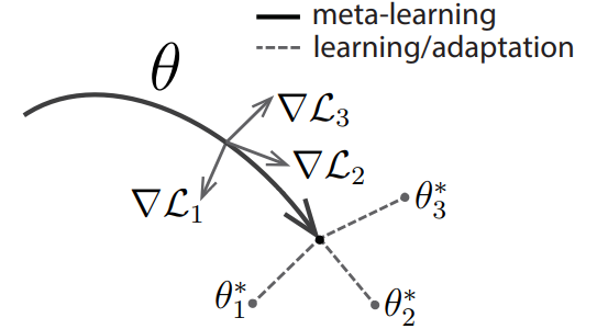
MAML의 최종 목적은 fast adaptation/finetuning (이하 FT) 이 가능한 위치로 model parameter $\theta$를 학습시키는 것입니다. 여기서 주목해야할 keywords는 “FT”입니다. MAML의 핵심 기작은 결국 “몇 step의 parameter update를 통해서 특정 task들에 도달할 수 있다면 효율적일 것이다!” 입니다. 예시를 들어 설명해보겠습니다. 만약 우리나라 전 지역을 돌아다녀야하는 직업을 가진 사람이라면 부산, 강릉, 인천 등에서 거주하는 것보다 대전에서 거주하는게 효율적일 것입니다. 이처럼, 모든 task를 일일이 학습하는 것보다 task에 빠르게 도달할 수 있는 위치로 $\theta$를 옮겨놓는게 다양한 task에 대해서 좋은 성능을 낼 수 있다는 것입니다.

위 문단에선 구구절절 말로 설명했다면 이번엔 수식적으로 보겠습니다. 들어가기에 앞서 MAML은 한 epoch을 학습하는데 inner-loop, outer-loop로 나뉘어집니다. inner-loop때는 위에서 언급한 FT, outer-loop는 model update$^*$입니다. MAML algorithm은 다음 Figure 1와 같습니다.

$^*$ 보통 이 과정을 bi-level optimization이라고도 합니다.

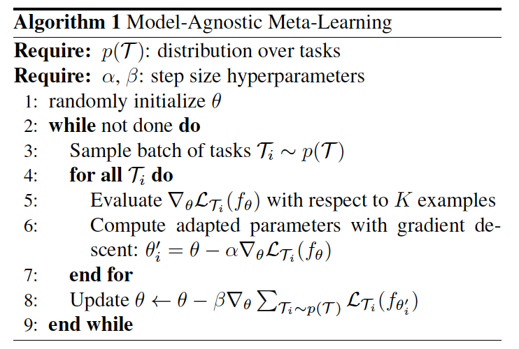그리고 위 pseudo-code를 풀어서 설명하면 다음과 같습니다:

1. Initialize model parameter $\theta$ (line 1)
2. Sample task $\mathcal{T}$ =($S$,$\mathcal{Q}$ ) ; $\mathcal{T} \sim p(\mathcal{T})$ along with the number of batches (line 3)
3. Inner-Loop updates with $n$ steps (line 4-7):
   1. Repeat SGD update: $\phi = \theta - \alpha\nabla_\theta \mathcal{L}(S;\theta)$
   2. $n \geq 2$부터는 $\theta$ → $\phi$ 으로 바뀜; 즉 $\phi = \phi - \alpha \nabla_\phi \mathcal{L}(\mathcal{S}; \phi)$ 같은 형태로 update
4. Outer-Loop (line 8):
   1. With fine-tuned model $\phi$, evaluate with $\mathcal{Q}$ and update
   2. $\Rightarrow$ $\theta \leftarrow \theta - \frac{1}{N}\sum_{i=1}^N \nabla_\theta \mathcal{L}_i(\mathcal{Q};\phi) $
5. Repeat 2-4 (line 2-9)

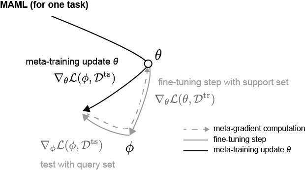
여기서 또 눈여겨보아야 할 부분은 outer loop 때의 derivative(meta-gradient) 입니다. 보면 outer loop update를 할 때 fine-tuned된 parameter $\phi$와 $Q$로 인해 나온 loss값을 $\phi$로 미분하는 것이 아닌 $\theta$으로 미분을 합니다. 관련 수식은 chain rule에 의해서 다음과 같이 전개됩니다.

\[\begin{aligned} \nabla_\theta \mathcal{L}(\mathcal{Q};\phi) &= \frac{\partial }{\partial \theta}\mathcal{L}(\mathcal{Q};\phi) \\ &= \frac{\partial \mathcal{L}(\mathcal{Q};\phi)}{\partial \phi} \frac{\partial \phi}{\partial \theta} \\ &= \nabla_\phi \mathcal{L}(\mathcal{Q};\phi)\nabla_\theta \phi \\ &=\nabla_\phi \mathcal{L}(\mathcal{Q};\phi)\nabla_\theta (\theta - \alpha \nabla_\theta \mathcal{L}(\mathcal{S};\theta)) \\ &= \nabla_\phi \mathcal{L}(\mathcal{Q};\phi)(I - \alpha \nabla^2_\theta \mathcal{L}(\mathcal{S};\theta)) \\ \end{aligned}\]

이 수식의 목적은 결국 최종적으로 $\theta$를 loss가 낮은 쪽으로 update 하자는 것인데, 그 방향을 FT된 $\phi$에서 loss $\mathcal{L}(\mathcal{Q};\phi)$를 낮추는 지점으로 update하자는 것입니다. 이 말이 모호하게 느껴질 수 있는데, Figure 2를 보시면 update 방향에 대해 어느정도 이해가 될 것 같습니다. (Reference: Boyang Zhao’s Blog, notation이 살짝 다른데 loss는 그냥 loss로 봐주시면 될 것 같습니다!!)

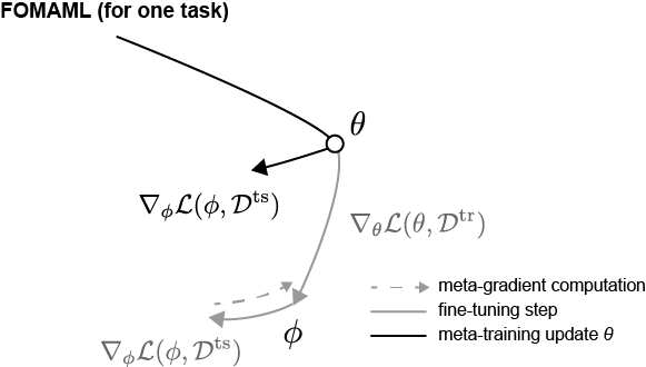
2.1.2 FOMAML, Reptile

MAML 같은 경우, hessian matrix multiplication($=\nabla_\theta^2 \mathcal{L}(\mathcal{S};\phi)$)이 들어가 있어 computational cost적인 관점에서 penalty가 있습니다. 그래서 성능을 어느정도 유지하면서 computational cost를 줄이는 방법들을 제시했습니다.

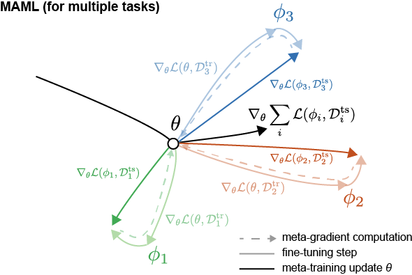
그 중 하나가 FOMAML (First-Order MAML) 입니다. FOMAML은 MAML 논문에서 실험적으로 확인한 것으로, hessian matrix를 무시한 채 학습을 진행해도 어느정도의 성능을 유지한다는 것입니다. 즉 $\nabla_\theta^2 \mathcal{L}(\mathcal{S};\phi) = 0$ 이라고 가정하는 것입니다. 관련해서 Figure 3에 잘 나타나 있는데, fintuning된 $\phi$ 에서 loss $\mathcal{L}(\mathcal{Q};\phi)$를 낮추는 “gradient의 방향”을 $\theta$ 에 적용하는 것입니다. 논문에서는 이 기작이 가능한 이유를 ReLU를 거치면서 hessian 값이 0으로 수렴하기 때문이라고 설명하고 있습니다. Loss landscape 관점에서 생각을 해보면, “loss를 낮추는 방향”이 비슷하다는 것입니다. 즉, 최종 update된 MAML에서의 $\theta$ 위치와 FOMAML에서의 $\theta$ 위치가 비슷한 loss landscape에 있다는 가정이 암묵적으로 들어가 있는 것이죠.

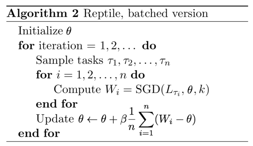
그 다음으로는 Reptile 논문입니다. Reptile 논문은 2018년에 OpenAI에서 발표한 논문으로, FOMAML의 variant 이라고 생각하시면 됩니다. Reptile의 특징은 $S$와 $Q$가 따로 존재하지 않습니다. Few-shot으로 학습하지만, task를 여러개 뽑아두고 sampling을 통해서 뽑은 task를 학습을 시킵니다. 그리고 initial model parameter $\theta$와 fine-tuned된 model parameter $\phi$ 차이를 gradient 삼아 update을 진행합니다. 아래에 Figure 4는 Reptile algorithm과 update 방향에 대한 그림입니다.

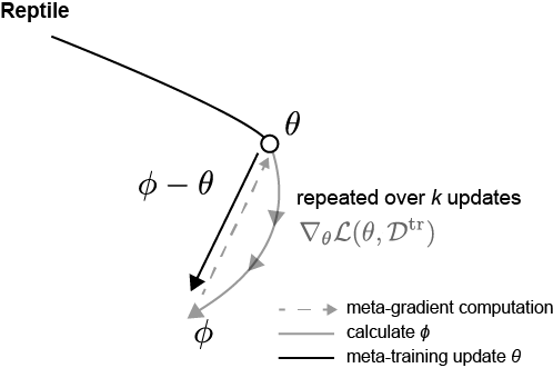기존 MAML 논문에 나온 notation과 달라서 헷갈릴수도 있는데, process를 풀어서 설명하면 다음과 같습니다.

1. Initialize model parameter $\theta$
2. Task $\mathcal{T}_i$ 를 $N$개 뽑는다. (where $\mathcal{T}_i \sim p(\mathcal{T})$, batch = $N$)
3. Inner Loop: 각 task $\mathcal{T}_i$별로 FT (fine-tuned parameters: $\phi_i$)
4. Outer Loop: $\theta$와 $\phi$의 차이만큼 $\theta$ update: $\theta \leftarrow \theta + \frac{\beta}{N}\sum_{i=1}^N (\phi_i - \theta)$
5. repeat 2-4

이와 같이 학습했을 때 결국 Reptile algorithm에서 meta-gradient의 expectation 값이 MAML의 meta-gradient와 비슷하게 수렴하게 됩니다. Reptile 논문의 대부분이 수학적으로 MAML, FOMAML과 어떻게 비슷하게 수렴하는지를 증명하는 내용입니다. 다만, 여기서는 간략하게 큰 맥락에서만 살펴보도록 하겠습니다. 이 역시 언젠가 기회가 된다면 증명 관련된 posting을 하도록 하겠습니다.

2.1.3 Wrap-up

Optimization-based Meta Learning은 few-shot learning을 할 때 gradient를 어떻게 활용하여 학습할지에 대한 meta learning approach 입니다. 다른 approach들과는 달리, gradient만 적절하게 설정한다면 다양한 분야에 model-agnostic하게 적용할 수 있다는 장점이 있습니다. 즉, Regression, classification, reinforcement learning 등 다양한 분야에 활용될 수 있습니다.

2.2 Metric-based Meta Learning

Metric-based meta learning은 말 그대로 거리 기반으로 similarity를 계산해 학습하는 개념입니다. 쉽게 얘기해 각 class 별로 가지고 있는 sementic 정보가 있을텐데, 그 sementic 정보간의 similarity를 통해 학습을 진행하게 됩니다. 어떻게 보면 $k$-NN 등과 같은 nearest neighbors의 개념과 비슷하다고 볼 수 있습니다. 대표적으로는 Matching Network, Prototypical Network, Relation Network가 있는데, 각 논문들에서 얘기하는 주요 개념들을 살펴보도록 하겠습니다. (Few-shot에 대한 개념을 계속 염두해두시면 좋을 것 같습니다!!)

2.2.1 Matching Network

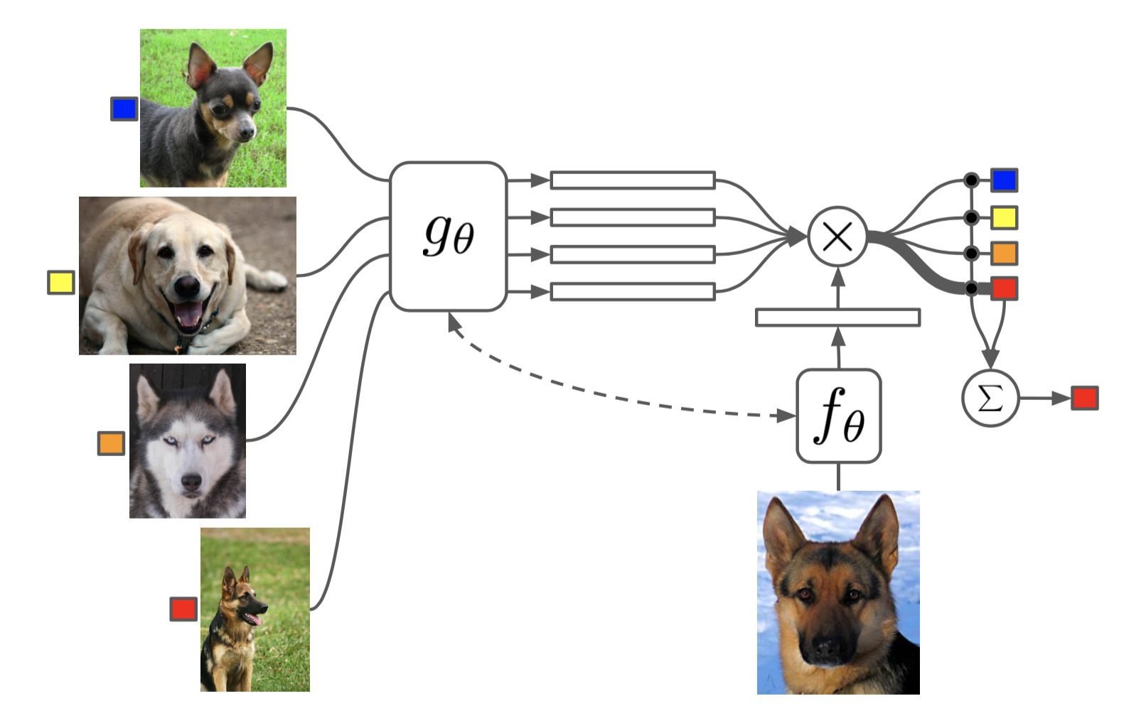
처음으로 볼 논문은 Matching Network입니다. Metric-based approach에서의 시초격인 논문입니다. 그 당시의 상황을 생각해보면, Transformer의 근간이 된 seq2seq 논문이 나왔습니다. Attention mechanism을 통해 extracted feature들만 보는 것이 아닌 전체적인 맥락, 즉 context를 통해 학습을 하자는 내용입니다. 따라서, 이 논문에서는 encoder를 통해 나온 feature간의 context를 비교를 하겠다는 겁니다.

우선 학습 process를 설명하기에 앞서, 이 논문에서는 최종 output에 대해서 설명합니다.

\[C_{\mathcal{S}}(\hat{\textbf{x}}) = P(y|\hat{\textbf{x}}, S) = \sum_{i=1}^k a(\hat{\textbf{x}}, \textbf{x}_i)y_i \; \;\; \text{where} \; \mathcal{S=\{ \text{(}\textbf{x}_i, y_i\text{)}\}_{i=1}^{k}}\]

위 수식은 attention mechanism을 가중치를 더 주는 것으로 활용을 하겠다는 의미입니다. 여기서 $a(\cdot, \cdot)$​은 attention kernel로 cosine similarity에 softmax를 취합니다:

\[a(\hat{x},x) =\frac{\exp(cos(f(\hat{x}), g(x)))}{\sum_{j=1}^k \exp(cos(f(\hat{x}), g(x_j)))}\]

위의 의미를 단순하게 해석해보면, 각 support sample $\textbf{x}_i $와 input $\textbf{x}$​에 대해서 attention kernel을 통해서 similarity를 계산 후 이를 가중치로 활용하여 비교 시 similarity가 더 높은 쪽으로 predict한다는 의미입니다. 여기서 input $\textbf{x}$는 query sample로 이해하시면 되겠습니다.

그렇다면 notation과 함께 학습 process를 보시겠습니다.

1. $g_\theta$​ 를 통해 support set의 feature representation vector 뽑기
2. $f_\theta$ 를 통해 query set의 feature representation vector 뽑기 (보통 $f_\theta = g_\theta$ )
3. 1과 2에서 나온 feature representation vector끼리 attention 값 구하기 $\rightarrow a(\cdot, \cdot)$
4. $C_\mathcal{S}$ 을 통해 query set의 label predict 하기

최근 논문들과 달리, meta learning 관련 초기 논문들에서는 few-shot setting을 context 관점에서 해결하기 위해 LSTM 구조를 활용했습니다. 그래서 이 논문에서도 LSTM 구조를 활용한 방법을 추가로 제시했습니다. ($\rightarrow$ Full Context Embeddings; FCE) LSTM model architecture를 어떻게 활용하는지 notation과 함께 FCE 학습 process를 보겠습니다.

• Embedding $g$
  • $g \rightarrow $ bidirectional LSTM, $g’ \rightarrow$​​​​ CNN (feature extractor)
  • $g(x_i, \mathcal{S})= \overrightarrow{h}_i + \overleftarrow{h}_i + g^\prime (x_i) $
  • $\overrightarrow{h}_i,\overrightarrow{c}_i = \text{LSTM}(g^{\prime} (x_i), {\overrightarrow{h}}_{i-1}, {\overrightarrow{c}}_{i-1})$ , $\overleftarrow{h}_i,\overleftarrow{c}_i = \text{LSTM}(g^{\prime} (x_i), {\overleftarrow{h}}_{i+1}, {\overleftarrow{c}}_{i+1})$
• $f \rightarrow$ LSTM , $f’ \rightarrow$ CNN (feature extractor)
  • $f(\hat{x}, \mathcal{S}) = \text{attLSTM}(f^\prime(\hat{x}), g(\mathcal{S}), K) $

$\Rightarrow k$ step에 따라…

1. $\hat{h}_k, c_k = \text{LSTM}(f^\prime (\hat{x}), [h_{k-1}, r_{k-1}], c_{k-1}) $​
2. $h_k = \hat{h}_k + f^\prime(\hat{x})$
3. $r_{k-1} = \sum_{i=1}^{|\mathcal{S}|}a(h_{k-1}, g(x_i))g(x_i)$
4. $a(h_{k-1}, g(x_i)) = \text{softmax}(h^\text{T}_{k-1}g(x_i))$

결국 여기서 LSTM을 사용하는 이유 각 feature vector들의 context를 더 잘 보기 위함인데, Omniglot 같은 쉬운 task에서는 성능 gain이 별로 없지만 $mini$-ImageNet 같은 조금 더 어려운 task에서는 성능 gain이 있습니다.

2.2.2 Prototypical Networks

그 다음 논문으로는 Prototypical Networks (이하 ProtoNet)입니다. 사실, metric-based meta learning 연구는 대부분 matching network보다 ProtoNet을 기반으로 생각하시면 됩니다.

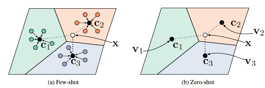
바로 본론으로 들어가겠습니다. ProtoNet은 각 label의 prototype vector와 feature vector들 간의 euclidean distance 연산을 통해서 학습을 진행합니다. 아래 Figure 6를 보시면, $c_n$들이 각 label의 prototype을 의미합니다. 그래서 새로운 task에 대해서 각 prototype과의 distance를 구하고 minimum distance인 prototype label로 mapping 시킵니다. 이 때 prototype은 support set을 통해 나온 feature vector의 평균으로 구합니다. 그렇다면 다음 학습 process를 통해서 좀 더 자세히 살펴보겠습니다.

• Notation (최대한 논문과 유사하게 설명드리겠습니다):
  • Support Set $\mathcal{S}_{n}= \{ (x_{n,j}^s, y_{n,j}^s) \}_{j=1}^{K}$, Query Set $\mathcal{Q}_{n}= \{ (x_{n,j}^q, y_{n,j}^q) \}_{j=1}^{Q}$​
  • $K$: support set 갯수 (a.k.a $K$-shot)
  • $Q$: query set 갯수
  • $c_n$: label $n$의 prototype $\rightarrow$ $\{c_1,\dots,c_N \}$, ($N$: $N$-way)
  • $f_\theta$ : Model parameterized by $\theta$​ (이하 feature extractor or backbone network)
  • loss $\mathcal{L}(\mathcal{D},c,\theta) = \frac{1}{|\mathcal{D}|}\sum_{(x,y)\in \mathcal{D}} l(-d(f_\theta(x), c),y)$,
    $\rightarrow$ loss function $l(\cdot, \cdot)$: Cross Entropy (CE), $-d(\cdot, \cdot)$: Euclidean Distance

1. $c_n = \frac{1}{| \mathcal{S}_n |} \sum_{j=1}^{| \mathcal{S}_n |} f_\theta (x^s_{n, j}) \Rightarrow $ support set으로 prototype vector ${c_n}$구하기
2. $\sum_{n=1}^{N}\mathcal{L}(Q_{n}, c_n, \theta) \Rightarrow$ query set과 prototype $c_n$​간 euclidean distance 구하기
3. $\theta \leftarrow \theta - \nabla_{\theta}\sum_{n=1}^{N}\mathcal{L}(Q_{n}, c_n, \theta)$ $\Rightarrow$ model parameter update

상당히 notation이 많고 복잡해서 이해하기 어려우실 수 있을거라 생각합니다. 만약 조금 과정이 복잡하시다면 그냥 단순하게 다음과 같이 이해하면 좋을 것 같습니다.

• Support Set으로 prototype이라는 label 만들기
• Query Set으로 prototype간의 거리 비교하기 $\Rightarrow$ Logits (최종 output)
• Query Set Label과 Logits간 CE 구하기
• CE로 parameter update하기

이 논문에서는 linear layer를 사용하지 않습니다. 어차피 feature vector를 거리 구하는데 직접적으로 사용하기 때문에 classification task임에도 불구하고 사용하지 않습니다. 다만, 이 논문에서는 euclidean distance를 하나의 linear model처럼 reinterpretation이 가능하다고 설명합니다. 다음 두개의 수식을 보면서 설명드리도록 하겠습니다.

\[-||f_\theta (x) - c_k||^2 = -f_\theta (x)^{\text{T}}\cdot f_\theta(x) +2c_k^{\text{T}}\cdot f_\theta(x) -c_k^{\text{T}}\cdot c_k \\\] \[2c_k^{\text{T}} \cdot f_\theta (x) - c_k^{\text{T}} \cdot c_k = w_k^{\text{T}}f_\theta(x) +b_k \;\; \text{where}\;\; w_k = 2c_k, \; b_k=-c_k^{\text{T}}c_k\]

사실 ProtoNet이 다른 distance metric 말고 euclidean distance를 고른 이유가 여기에 있습니다. Deep Learning의 기본 concept은 backbone network가 feature representation을 원활하게만 한다면 나머지는 상황에 맞게 (특히 classification task) linear transformation만 해주면 됩니다. 보통 이런 과정을 deep learning에서는 learnable한 linear layer를 backbone network 뒤에 붙여서 학습을 합니다. 그런데 ProtoNet은 euclidean distance를 통해 학습을 진행하면 이런 linear transformation 과정을 내포하고 있다고 해석하고 있습니다. 또한, euclidean distance가 적절하다고 가정을 할 수 있는 이유 중 다른 하나는 학습 시 non-linearity가 필요한 부분은 이미 backbone network를 통해서 다 학습했기 때문이라고 주장하고 있습니다. (이런…. assume이 꼭 필요한 부분인지는 잘 모르겠습니다…)

(진짜 마지막으로…) 이렇게 reinterpret 했을 때 또 다른 장점은 ProtoNet에 MAML (이하 Proto-MAML)을 적용할 수 있다는 점입니다. $w_k^{\text{T}}f_\theta(x) +b_k$​ 가 linear layer 역할을 하기 때문에 FT가 가능해집니다. Proto-MAML 학습 process에 대해 (짧게) 설명하겠습니다.

• Notation:
  • $f_\theta$: backbone network
  • $g_\theta(x_i) = w_{i,k}^{\text{T}}f_\theta(x_i) +b_k$
  • Loss $\mathcal{L}(\mathcal{D};\theta) = \frac{1}{|\mathcal{D}|}\sum_{(x,y)\in\mathcal{D}}l(g_\theta(x), y)$

1. Inner Loop
   1. support set $\mathcal{S}_i$ 을 통해 prototype $c_{i,k}$ 구하기
   2. $\phi = \theta - \alpha \nabla_\theta \mathcal{L}(\mathcal{S}_i;\theta)$
   3. $n$ step 반복하기
2. Outer Loop: $\theta \leftarrow \theta - \frac{\beta}{\mathcal{B}}\sum_{i=1}^{\mathcal{B}}\nabla_\theta \mathcal{L}(\mathcal{Q}_i;\phi)$

실제로 논문 중 (fo-)Proto-MAML을 제시한 논문이 있습니다. 읽어보시면 논문상에서 아주 main concept은 아니지만 Proto-MAML이 성능향상이 있다는 것을 보여줬습니다.

*마치며

이 글까지 meta-learning의 시초가 되는 논문들을 거의 다 다룬 것 같습니다. 설명한 위 논문들이 나온 2016년, 2017년 이후에 한 4-5년간 폭발적으로 meta-learning 연구들이 이루어졌고, 지금은 약간 감소되긴 했지만 그래도 꾸준하게 top-conference 논문들에 게재되고 있습니다. 다만, 이제는 meta-learning이라는 algorithm 자체를 연구하는 것이 아닌 다른 연구들에 접목시키는 방향으로 바뀐 추세입니다. 특히, foundation model 연구가 굉장히 활발해지면서, 소수 data로 학습을 할 수 있는 few-shot 개념이 더욱 중요해진 것 같네여… (AI분야의 성장속도가 너~~무 빠르네여…. 😂🥲

다음 주제로는 제가 이제 막 시작한 foundation model (LLM, LVM 등)에 대해서 논문리뷰든, 컨셉이든 posting해볼까 생각합니다. 세부 주제를 어디 쪽으로 잡을지 잘 모르겠지만 어느정도 공부가 된 후 다시 찾아오겠습니다. 부족한 글 끝까지 읽어주셔서 매우매우 감사합니당!! :) 😁🫡