$\star$ First, before explaining, I will omit what convex/non-convex is, and the overall formulas within deep learning. They are explained so well in other blogs, so is there a need? However, here I will try to focus more on “Why?”, or “How?”. Especially, I will try to focus more on the formula derivation.
Why Convex Optimization?
Most problems we actually have to solve are in non-convex forms. However, solving such non-convex functions requires more precise approximation and proof. In this case, the cost becomes too large and it can be inefficient. But if we solve it assuming that the corresponding function is convex within the range we can assume, we can solve it efficiently. In other words, if we assume an arbitrary function $f$ is convex, since the local minima for $f$ is the global minima, the task to solve becomes relatively very easy because we only need to find the local minima. Then let’s take a look through simple examples.
The Taxonomy below represents the classification criteria during optimization. $\star$ Taxonomy:
- Zeroth Order: Only value of Function
- $1^{st}$ Order: Derivation (GD/ SGD/ mini-batch GD, etc.)
- $2^{nd}$ Order: Hessians (Newton Methods, etc.)
Example: Gradient Descent
One of the most basic methods to find the optimal solution in the Deep Learning field is Gradient Descent (hereinafter, GD). Actually, nowadays most people use other optimization techniques (e.g., SGD, Adam, etc.) instead of GD, but if you understand how GD converges from an optimization perspective, I think you will be able to understand the other techniques sequentially.
Then, let’s look at how optimization is performed for GD, and how the convergence form of optimization changes according to assumptions. (All assumptions here are based on convex)
Problem Formulation 1
(Assumption: $L$-Lipschitz)
Before we dive in, optimization settings are usually established briefly as follows:
\[\min\limits_{x \in \mathbb{R}^d} f(x)\]where $f$ is differentiable convex function.
And since GD is, as everyone knows, an iterative algorithm, it can be written as follows:
\[x_{k+1} = x_k -\gamma \nabla f(x_k)\] where $\gamma > 0 $ is the step size, a.k.a learning rate
Then, to find the optimal solution, we will repeat the above content continuously. Assuming that training proceeds without diverging, a good optimization algorithm is a battle of how fast it finds the optimal solution. If asked “How do we find this?”, we can find it through upper bound settings for the final step $T$. In other words, when training has finally proceeded:
Theorem 1: Let $f$ be convex and $L$-Lipschitz continuous. Then gradient descent with $\gamma = \frac{\mid\mid x_1 - x^\star\mid\mid}{L\sqrt{T}}$ satisfies:
\[f \left ( \frac{1}{T} \sum_{k=1}^T x_k \right) - f(x^{\star}) \leq \frac{|| x_1 - x^\star || L}{\sqrt{T}} \Rightarrow \mathcal{O}(\frac{1}{\sqrt{T}})\]Proof:
First, to solve the problem, we can use a method of projecting onto convex sets. In other words, when projecting onto convex sets, the inner product of $x$ and $z$ with respect to the projection position $\pi_c (z)$ always results in a negative number (obtuse angle), and if we utilize the Pythagorean theorem, the inequality $\mid\mid \pi_c (z) - x\mid\mid \leq \mid\mid z - x \mid\mid$ holds true. Also, later during the proof derivation, I plan to utilize the Pythagorean theorem as follows: $\mathbf{\left<a,b\right> = \frac{1}{2}(\mid\mid a\mid\mid^2 + \mid\mid b\mid\mid ^2 -\mid\mid a-b\mid\mid ^2)}$)
Then, using the properties above, let’s develop the proof:
\[\begin{align} f(x_k) - f(x^\star) &\leq \; \;\left<\nabla f(x_k) \;, \; x_k - x^\star \right> \; \rightarrow \text{1st order convexity}\\ &= \; \left<-\frac{1}{\gamma}(x_k - x_{k+1}) \;,\; x_k - x^\star\right> \; \rightarrow \text{$x_{k+1} - x_k = - \gamma \nabla f(x_k)$ }\\ &= \frac{1}{2\gamma} \left[ \; \mid\mid x_k - x_{k+1}\mid\mid ^2 + \mid\mid x_k - x^\star\mid\mid ^2 - \mid\mid (x_k - x_{k+1}) - (x_k - x^\star)\mid\mid ^2 \; \right] \rightarrow \; \text{pythagoras theorem}\\ &=\frac{1}{2\gamma} \left[ \; \mid\mid x_k - x^\star\mid\mid ^2 +\mid\mid \gamma \nabla f(x_k)\mid\mid ^2 - \mid\mid x_{k+1}- x^\star\mid\mid ^2 \; \right] \\ &= \frac{1}{2\gamma} \left[ \; \mid\mid x_k - x^\star\mid\mid ^2 - \mid\mid x_{k+1} - x^\star\mid\mid ^2 \right] + \frac{\gamma}{2} \mid\mid \nabla f(x_k)\mid\mid ^2 \end{align}\]Here, the $L$-Lipschitz Continuity property: if $f$ is differentiable, then $\mid \nabla f (x) \mid \leq L$. $\rightarrow$ Using $\frac{\gamma}{2} \mid\mid \nabla f(x_k)\mid\mid ^2 \leq \frac{\gamma L^2}{2}$, we can set the bound as follows.
\[\begin{align} \frac{1}{2\gamma} \bigg [ \; \mid\mid x_k - x^\star\mid\mid ^2 - \mid\mid x_{k+1} - x^\star\mid\mid ^2 \bigg] + \frac{\gamma}{2} \mid\mid \nabla f(x_k)\mid\mid ^2 \\ \leq \frac{1}{2\gamma} \bigg [ \; \mid\mid x_k - x^\star\mid\mid ^2 - \mid\mid x_{k+1} - x^\star\mid\mid ^2 \bigg] + \frac{\gamma}{2} L^2 \end{align}\]Now, let’s substitute the $k$ values sequentially and expand the formula.
\[\begin{align} f(x_1) - f(x^\star) &\leq \frac{1}{2\gamma} \bigg [ \; \mid\mid x_1 - x^\star\mid\mid ^2 - \mid\mid x_{2} - x^\star\mid\mid ^2 \bigg] + \frac{\gamma L^2}{2} \\ f(x_2) - f(x^\star) &\leq \frac{1}{2\gamma} \bigg [ \; \mid\mid x_2 - x^\star\mid\mid ^2 - \mid\mid x_{3} - x^\star\mid\mid ^2 \bigg] + \frac{\gamma L^2}{2} \\ &\;\;\vdots \\ f(x_k) - f(x^\star) &\leq \frac{1}{2\gamma} \bigg [ \; \mid\mid x_k - x^\star\mid\mid ^2 - \mid\mid x_{k+1} - x^\star\mid\mid ^2 \bigg] + \frac{\gamma L^2}{2} \\ &\;\;\vdots \\ \end{align}\]If we take the average for both hand sides of the Inequality:
\[\frac{1}{T} \sum_{k=1}^T \bigg[ f(x_k) - f(x^\star)\bigg] \leq \frac{1}{T*2\gamma} \bigg[ ||x_1 - x^\star||^2 - ||x_{T+1} - x^\star||^2 \bigg] + \frac{\gamma L^2}{2}\]Here, since $\mid\mid x_{T+1} - x^\star\mid\mid ^2$ has a $-$ attached in front, this term is always negative. Therefore, we can just eliminate it and set an additional upper bound.
\[\Rightarrow \frac{1}{T*2\gamma} \left[ || x_1 - x^\star || ^2 - || x_{T+1} - x^\star || ^2 \right] \leq \frac{1}{T*2\gamma} \cdot || x_1 - x^\star || ^2\]And then, *utilizing Jensen’s Inequality, we can express it as $f(\frac{1}{T} \sum_{k=1}^Tx_k) \leq \frac{1}{T} \sum_{k=1}^Tf(x_k)$. (Since we already assumed $f$ is convex)
*Jensen’s Inequality: If $f$ is convex, it satisfies $f(\mathbb{E}[x])\leq \mathbb{E}[f(x)]$.
Expanding the formula according to this gives:
\[\begin{align} f(\frac{1}{T} \sum_{k=1}^Tx_k) - f(x^\star) &\leq \frac{1}{T} \sum_{k=1}^Tf(x_k) - f(x^\star) \leq \frac{\mid\mid x_1 - x^\star\mid\mid ^2}{2\gamma T} + \frac{\gamma L^2}{2} \\ \Rightarrow f(\frac{1}{T} \sum_{k=1}^Tx_k) - f(x^\star) &\leq \frac{\mid\mid x_1 - x^\star\mid\mid ^2}{2\gamma T} + \frac{\gamma L^2}{2} \\ \end{align}\]Finally, if we substitute the step size $\gamma = \frac{\mid\mid x_1 - x^\star\mid\mid}{L\sqrt{T}}$
\[\begin{align} f(\frac{1}{T} \sum_{k=1}^Tx_k) - f(x^\star) &\leq \frac{|| x_1 - x^\star|| ^2}{2\gamma T} + \frac{\gamma L^2}{2} \\ &= \frac{L \sqrt{T}}{|| x_1 - x^\star|| } * \frac{|| x_1 - x^\star|| ^2}{2 T} + \frac{L^2|| x_1 - x^\star || }{2*L \sqrt{T}} \\ &= \frac{L\sqrt{T}(|| x_1 - x^\star || )}{2T} + \frac{L\sqrt{T}(|| x_1 - x^\star || )}{2T} \\ &= \frac{L || x_1 - x^\star|| }{\sqrt{T}} \end{align}\]When expanded like this, we can see it comes out identical to Theorem . This means that the convergence rate varies according to $T$, and assuming $f$ is convex and $L$-Lipschitz, that speed converges to $\mathcal{O}\left(\frac{1}{\sqrt{T}}\right)$.
Side Note: Fixed Step Size vs. Adaptive Step Size
If you look at other textbooks, papers, blogs, etc., when proving Gradient Descent, they often set a fixed step size $\gamma = \frac{1}{L}$ and derive it. Actually, when done this way, it is quite neat mathematically and the convergence rate is also faster at $\mathcal{O}(\frac{1}{T})$. However, when proceeding like this, because you have to set a constant value, and when expanding the formula, if it is a fixed step size, an independent term regarding $\frac{1}{T}$ is created in the bound RHS, so you cannot guarantee it really goes to the minimum. Therefore, you can understand the method I developed as giving up the convergence rate to set a step size dependent on the difference between the actual first input $x_1$ and optimal $x^\star$ and the number of iterations $T$, to make a slightly more adaptive step size.
(Since the proof for Fixed Step Size is available so widely, I will omit it)
Afterwards…
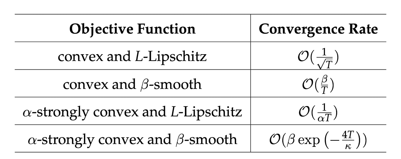
The derivation above is a formula developed assuming $f$ is convex and $L$-Lipchitz continuous. If the assumption becomes stronger ($\beta$-smooth, $\alpha$-strongly convex, etc.), the convergence rate changes. Future postings will proceed by proving the convergence rate according to assumptions.
I will finish by introducing the convergence rate table according to assumptions for GD.
$*$Thank you very much for reading. If there are any incorrect parts while reading or if you have any advice, I would appreciate it if you could share your opinions anytime.